Showcases
Our add-on pulse compressors are compatible with different ultrafast industrial lasers. Here we experimentally prove this compatibility and demonstrate outstanding performance.
MIKS1_S
@ FemtoLux 30
(EKSPLA)
MIKS1_S @ Pharos (Light Conversion)
​
In this section we present the performance of our MIKS1_S module with PHAROS driver laser. The compressed output pulses reach 40 fs in duration with over 90 % power transmission. Starting from 230 fs input pulses this corresponds to an increase in peak power up to 2 GW. Text-book-like self-phase modulated spectrum and excellent pulse compression are shown in the pictures below.
​
Input Pharos: 230 fs, 95 uJ, 9.5 W
Output MIKS1_S: 40 fs, 89 uJ, 8.9 W
​
Input spectrum vs. output spectrum
​
Input autocorrelation vs output autocorrelation
​
Positional stability
​
The centroid of the beam cross section was tracked over 1 hour ca. 1 meter behind the output aperture of MIKS1_S. Note that the standard deviation of the centroid fluctuation is smaller than 1% of the beam diameter (1/e2).
Output power stability
​
Output spectrum stability
​
MIKS1_S @ TruMicro 2030 (Trumpf Laser)
​
Here we show the performance of our MIKS1_S module driven by TruMicro2030 fiber laser. By increasing the bandwidth to over 45 nm, a pulse duration of 52 fs could be achieved with a transmission of over 90%.
Input TruMicro 2030: 950 fs, 50 uJ, 10 W
Output MIKS1_S: 52 fs, 45 uJ, 9 W
​
​
Input spectrum vs. output spectrum
​
Input autocorrelation vs. output autocorrelation
​
MIKS1_S @ FemtoFiber vario 1030 (TOPTICA Photonics)
​
In this section we present the performance of our MIKS1_S module with FemtoFiber vario 1030 driver laser. The compressed output pulses reach 40 fs in duration with over 90 % power transmission. Starting from 200 fs input pulses this corresponds to an increase in peak power of factor 4. The self-phase modulated spectrum and the pulse compression are shown in the graphs below.
​
Input FemtoFiber Vario: 200 fs, 10 μJ, 10 W
Output MIKS1_S: 40 fs, 9 μJ, 9 W
Input spectrum vs. output spectrum
​
Input autocorrelation vs. output autocorrelation
​
MIKS1_S @ neoMOS SMAART (neoLASE)
​
Here we show the performance of our MIKS1_S module driven by neoLASE neoMOS SMAARTlaser. A peak power increase by a factor of seven could be achieved with an efficiency of over 90%. The self-phase modulated spectrum and the pulse compression are shown in the graphs below.
​
Input neoMOS SMAART: 900 fs, 170 μJ, 52 W
Output MIKS1_S: 100 fs, 155 μJ, 47 W
​
Input spectrum vs. output spectrum
​
Input autocorrelation vs. output autocorrelation
​
MIKS1_S @ INDYLIT 10 (Litilit)
​
Here we show the performance of our MIKS1_S module driven by INDYLIT 10 solid state laser. The compressed output pulses reach 50 fs in duration with over 90 % power transmission. Starting from 420 fs input pulses this corresponds to an increase in peak power of factor 6. The self-phase modulated spectrum and the pulse compression are shown in the graphs below.
​
Input INDYLIT 10: 420 fs, 100 μJ, 10 W
Output MIKS1_S: 50 fs, 93 μJ, 9.3 W
​
Input spectrum vs. output spectrum
​
Input autocorrelation vs. output autocorrelation
​
MIKS1_S @ Carbide (Light Conversion)
Here we show the performance of our MIKS1_S module driven by Carbide laser. A peak power increase by a factor of 4 could be achieved with an efficiency of over 98%. The self-phase modulated spectrum and the pulse compression are shown in the graphs below.
​
Input Carbide: 200 fs, 15 μJ, 6 W
Output MIKS1_S: 52 fs, 14.7 μJ, 5.9 W
Input spectrum vs. output spectrum
​
Input autocorrelation vs. output autocorrelation
​
Output beam profile
​
MIKS1_S @ FemtoLux 30 (EKSPLA)
Here we show the performance of our MIKS1_S module driven by EKSPLA laser. A peak power increase by a factor of 7 could be achieved with an efficiency of over 90%. The self-phase modulated spectrum and the pulse compression are shown in the graphs below.
​
Input FemtoLux 30: 350 fs, 100 μJ, 20 W
Output MIKS1_S: 50 fs, 90 μJ, 18 W
Input spectrum vs. output spectrum
​
Output beam profile
​
Typical FROG trace
​
MIKS1_S @ Monaco (Coherent)
​
Here we show the performance of our MIKS1_S module driven by Monaco femtosecond laser. A peak power increase by a factor of 6 could be achieved with an efficiency of over 95%. The self-phase modulated spectrum and the pulse compression are shown in the graphs below.
​
Input Carbide: 320 fs, 80 μJ, 60 W
Output MIKS1_S: 52 fs, 77 μJ, 58 W
Input spectrum vs. output spectrum
​
Input autocorrelation vs. output autocorrelation
​
Output beam profile
​
MIKS1_L @ A2000 (Amphos)
​
Here we show the performance of our MIKS1_L module driven by Amphos laser. The compressed output pulses reach 82 fs in duration with 85 % power transmission. Starting from 1 ps input pulses this corresponds to an increase in peak power of factor 10. The self-phase modulated spectrum and the pulse compression are shown in the graphs below.
​
Input Amphos: 1 ps, 1 mJ, 100 W
Output MIKS1_S: 82 fs, 850 μJ, 85 W
​
Input spectrum vs. output spectrum
​
Input autocorrelation vs. output autocorrelation
​
Output beam profile
​
MIKS12 @ Pharos (Light Conversion)
​
In this section we present the performance of our MIKS12 module with PHAROS driver laser. The compressed output pulses reach sub 20 fs in duration with over 85 % power transmission. By increasing the bandwidth to over 200 nm, a pulse duration of 17 fs could be achieved.
Input PHAROS: 260 fs, 20 uJ, 60 kHz
Output MIKS12: 17 fs, 16.4 uJ, 60 kHz
​
Output spectrum
​
Output autocorrelation
​
MIKS12_UP @ Pharos (Light Conversion)
​
Here we show the performance of our MIKS12_UP module driven by Pharos laser. The compressed output pulses reach 7 fs in duration with 83 % power transmission. Starting from 230 fs input pulses this corresponds to an increase in peak power of factor 27. The self-phase modulated spectrum and the pulse compression are shown in the graphs below.
​
Input Pharos: 230 fs, 12 uJ, 1 MHz
Output MIKS12_UP: 7 fs, 10 uJ, 1 MHz
​
Input spectrum vs. output spectrum
​
Input autocorrelation vs. output autocorrelation
​
MIKS1_XS @ TruMicro 2030 (Trumpf Laser)
​
Here we show the performance of our MIKS1_XS module driven by TruMicro 2030 femtosecond laser. A peak power increase by a factor of 3.5 could be achieved with an efficiency of over 80%. The self-phase modulated spectrum and the pulse compression are shown in the graphs below.
​
Input TruMicro 2030: 280 fs, 1 uJ, 1.2 W, 1 MHz
Output MIKS1_XS: 61 fs, 0.8 uJ, 0.9 W, 1 MHz
Input spectrum vs. output spectrum
​
Input autocorrelation vs. output autocorrelation
​
MIKS1_S @ Dira 200-100 (Trumpf Scientific Laser)
​
In the following we present the results obtained from our MIKS1_S module, which was powered by the Dira 200-100 femtosecond laser. We successfully achieved a significant peak power increase of over 11 times, while maintaining an impressive efficiency rate exceeding 95%. The graphs below illustrate the self-phase modulated spectrum and the pulse compression achieved through our experiments.
​
Input Dira 200-100: 1.000 fs, 200 uJ, 20 W, 100 kHz
Output MIKS1_S: 92 fs, 190 uJ, 19 W, 100 kHz
Input spectrum vs. output spectrum
​
Input autocorrelation vs. output autocorrelation
​
Output beam profile
​
MIKS1_XS @ Ti:Sa Laser (Simulations)
​
Here we show the potential performance of our MIKS1_XS module driven by a Titanium Sapphire femtosecond laser. We consider relatively short 40 fs pulses at the input of our pulse compressor. A peak power increase by a factor of 4.6 could be achieved with an efficiency of over 90%. Essentially it means that we can use broadband dispersive dielectric mirrors in this case. The spectrum before and after the compressor as well as the theoretically compressed output pulses of 8.3 fs are shown below. Of course, it would also be possible to have stronger or weaker self-phase modulation and this way get even shorter or longer pulses.
​
Titanium Sapphire Laser: 40 fs, 5 uJ, 250 kHz
Output MIKS1_XS: 8.3 fs, 4.8 uJ, 250 kHz
Simulated Input spectrum vs. output spectrum
​
Simulated Input autocorrelation vs. output autocorrelation
​
Dispersion Compensation for Micromachining Setup
Here we show the performance of our MIKS1_S module driven by Carbide laser. A peak power increase by a factor of 4 could be achieved with an efficiency of 95%. The self-phase modulated spectrum and the pulse compression are shown in the graphs below.
​
On top of that we compensated the addtional dispersion introduced by the optics from the micromachining setup. This way we could achieve sub 100 fs pulse duration at the actual workpiece.
​
Laser pulses experience chromatic dispersion, i. e. varying group velocities for different wavelengths, while propagating through material. This effect stretches the pulses in the time domain. In general, shorter pulses with a wider spectrum are more susceptible to this effect. Commonly used micromachining setups comprise multiple such elements, for example beam expanders or f-theta lenses. It is thus necessary to account for the dispersion to benefit from ultrashort laser pulses on the workpiece.
​
Input Carbide: 400 mW, 40 µJ, 10 kHz, 230 fs
Output MIKS1_S: 380 mW, 38 µJ, 10 kHz, 50 fs
​
Additional micromachining setup:
-
Beam expander
-
Galvo-Scanner
-
F-Theta-Lens
Output spectrum after micromachining setup
​
Output pulse duration after micromachining setup
​
Output beam profile after micromachining setup
​
MIKS1_L @ Pharos (Light Conversion)
​
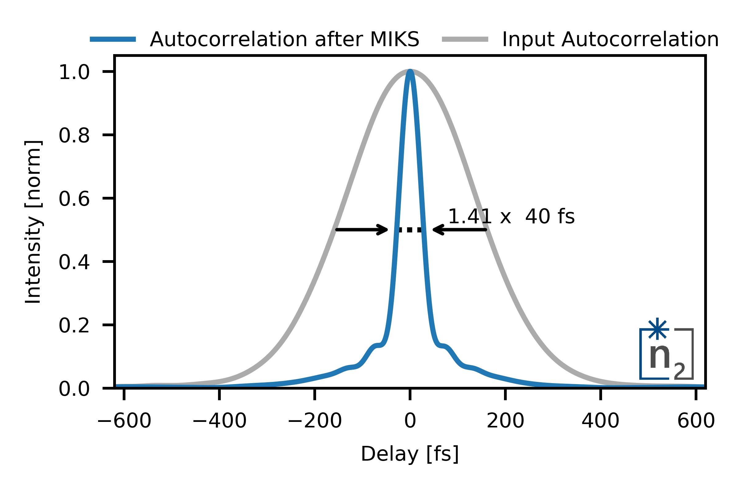
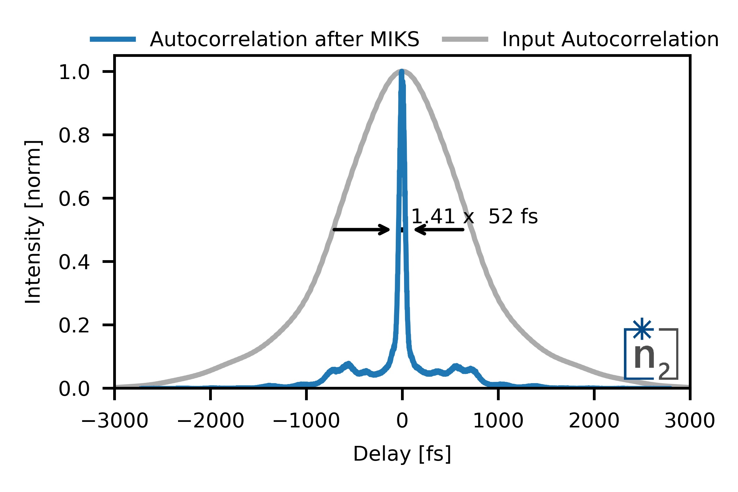
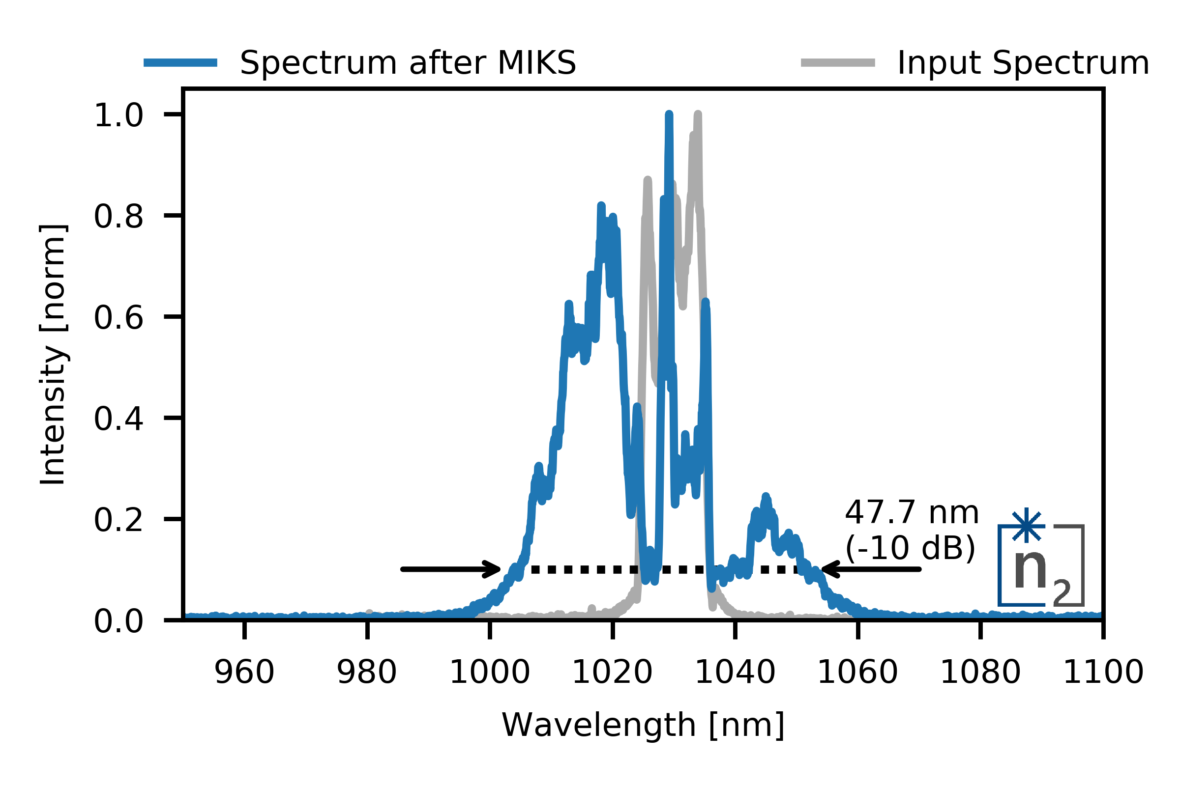
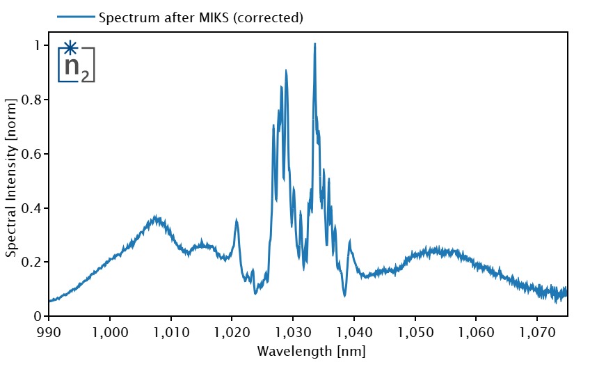
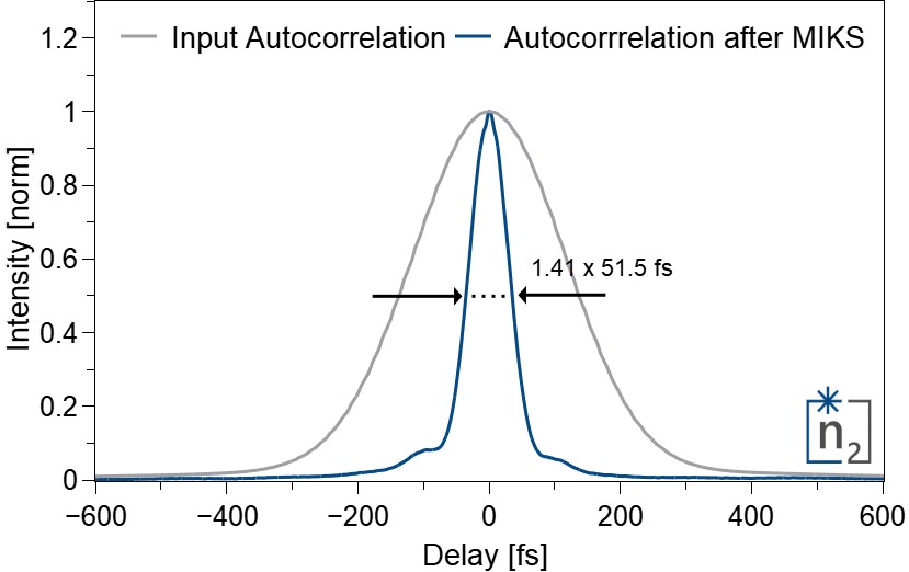
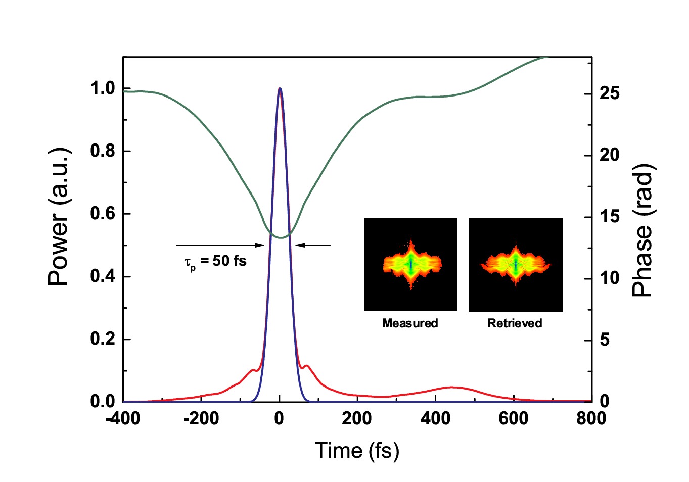
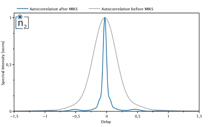
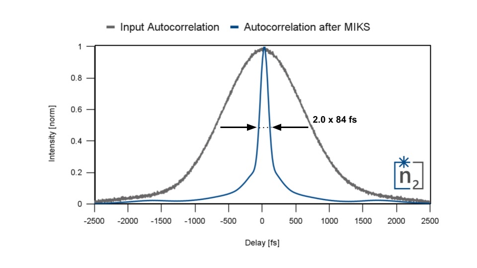
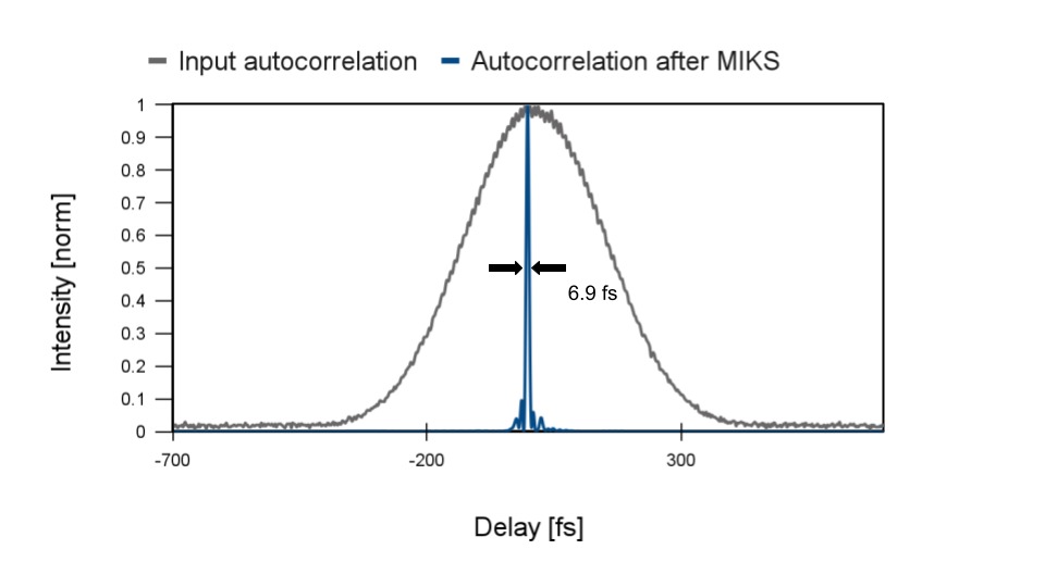
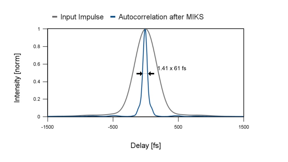
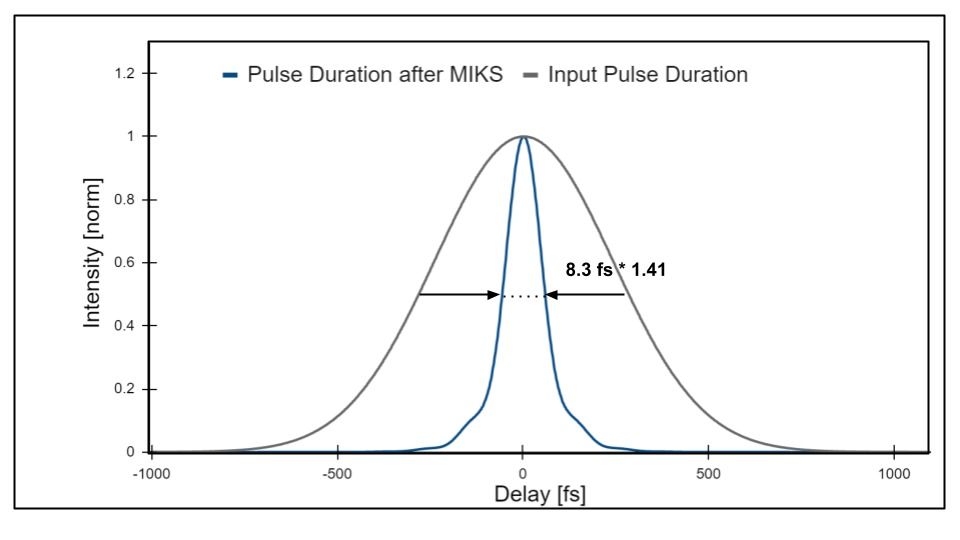
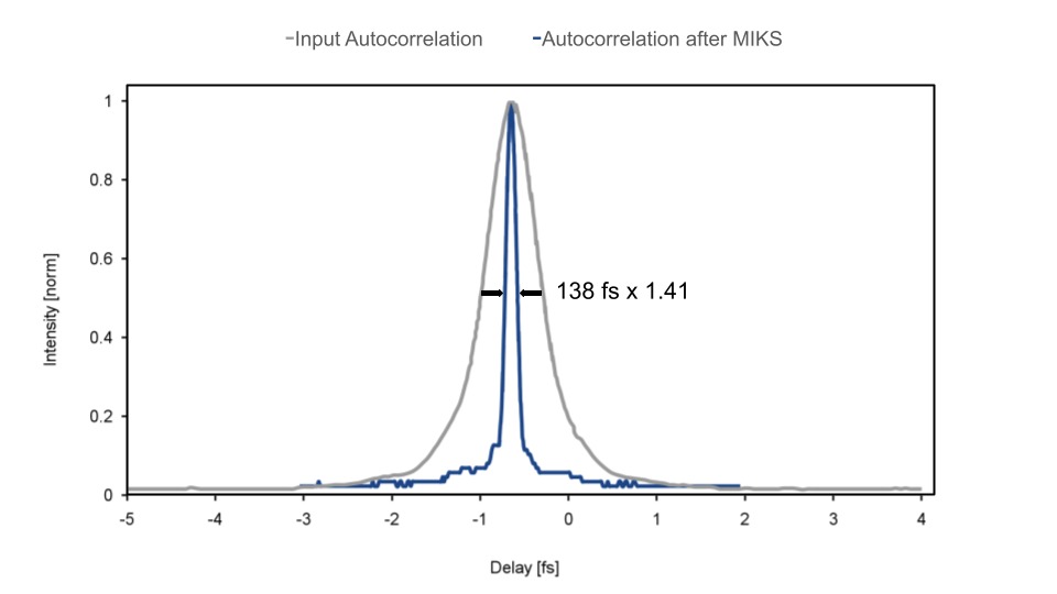
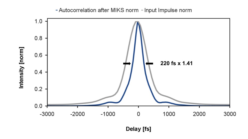
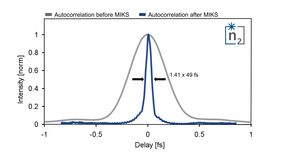
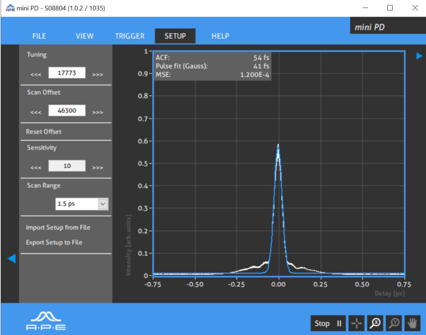
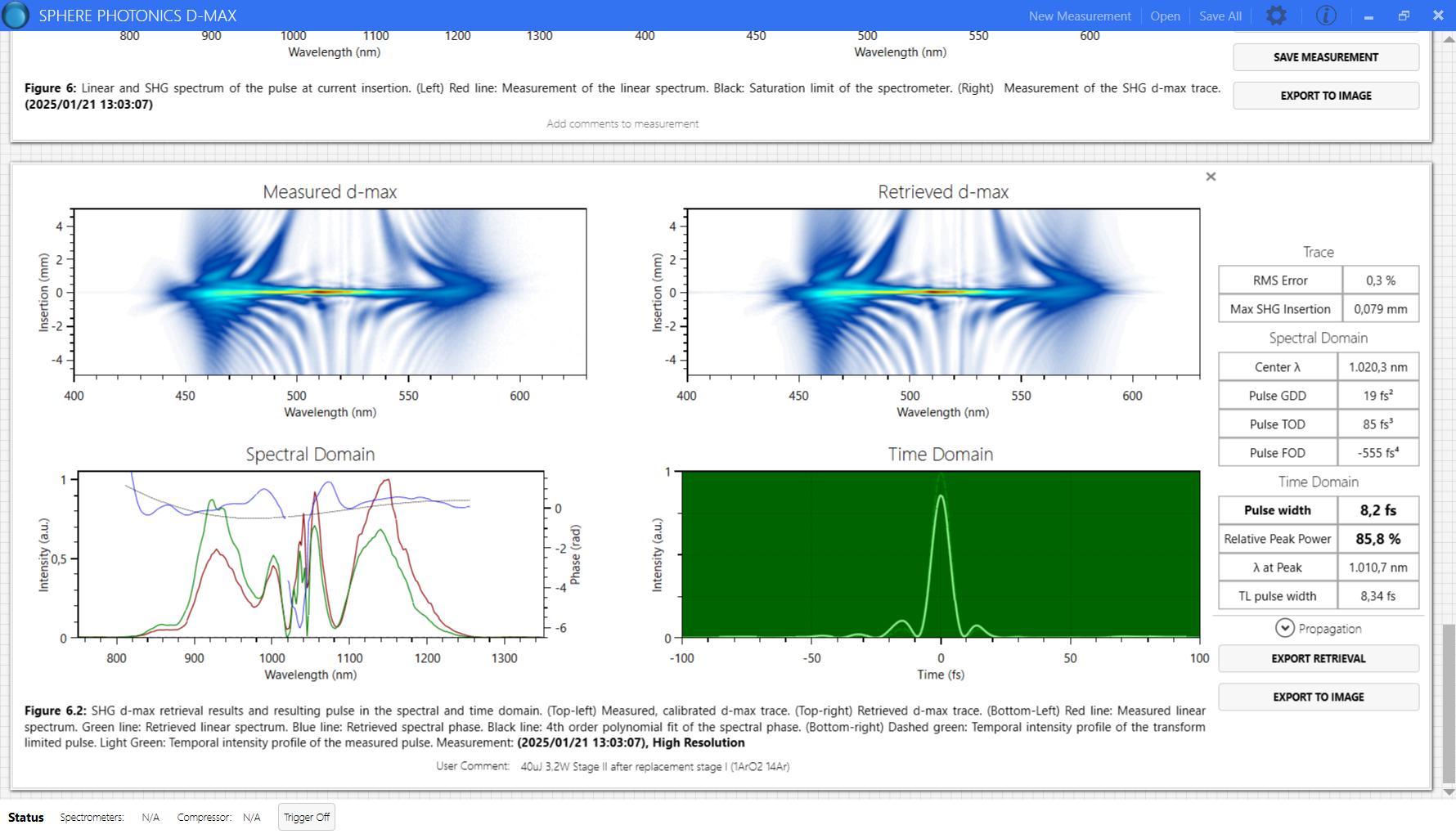
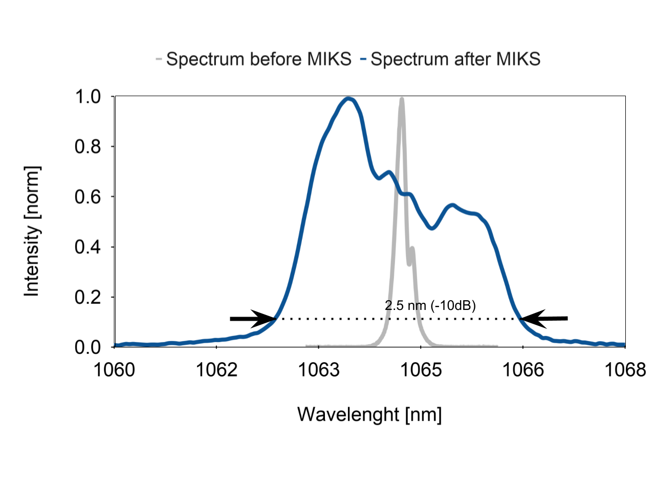
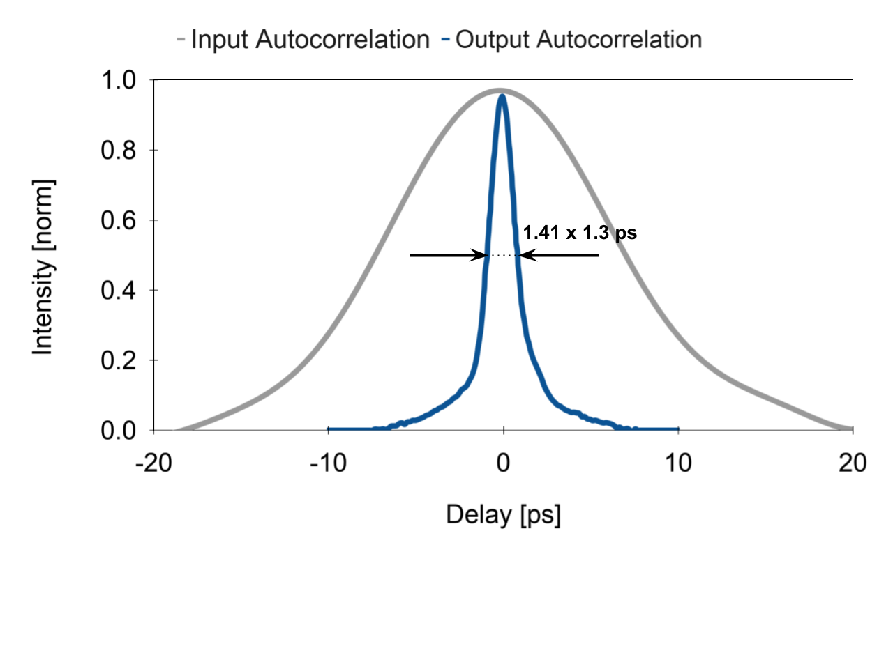
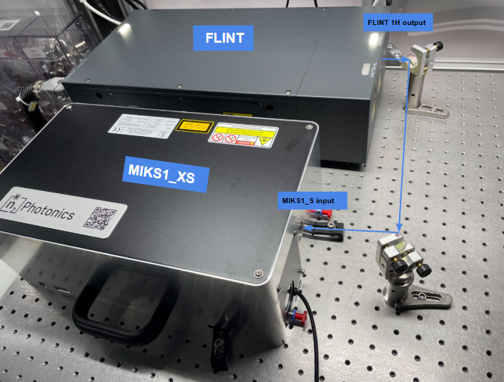
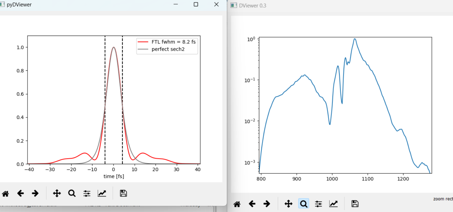
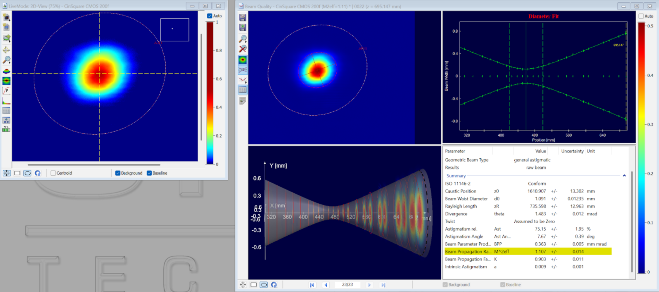
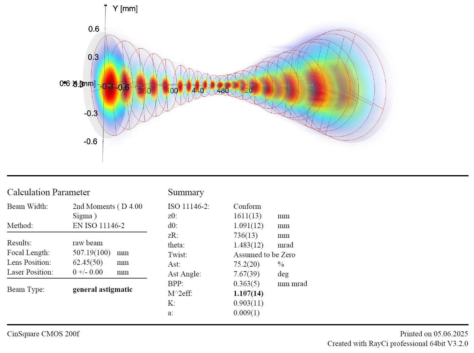
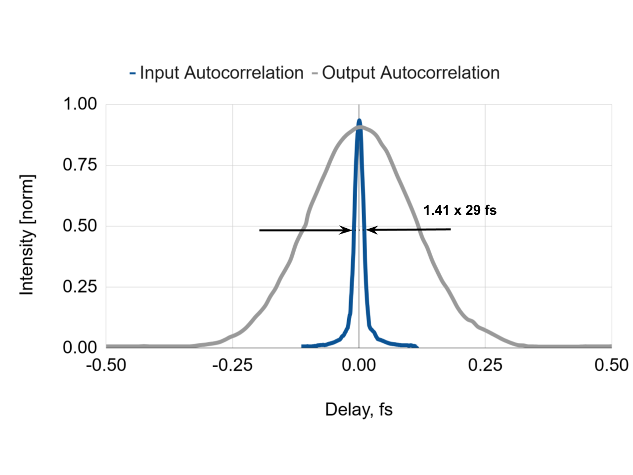
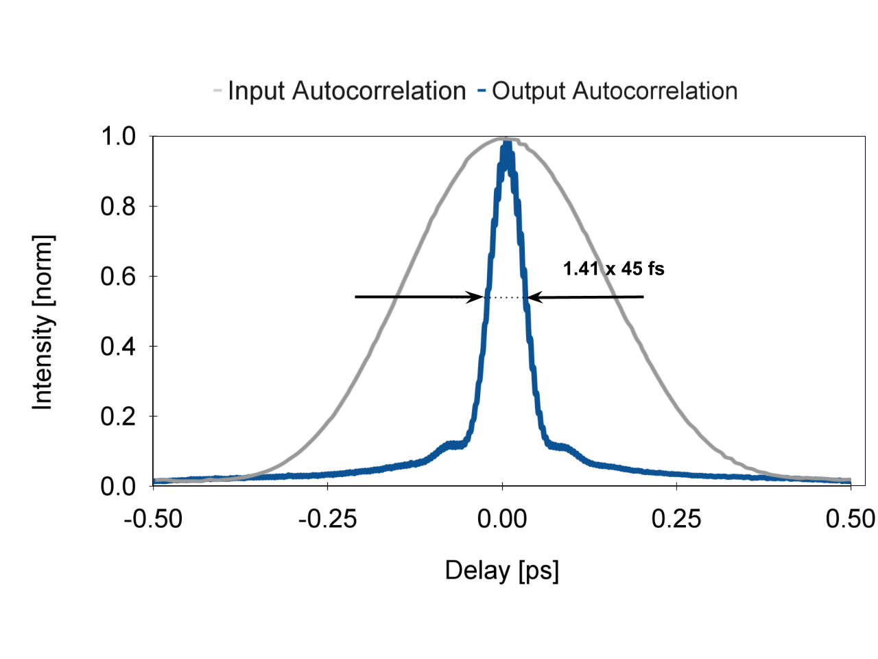
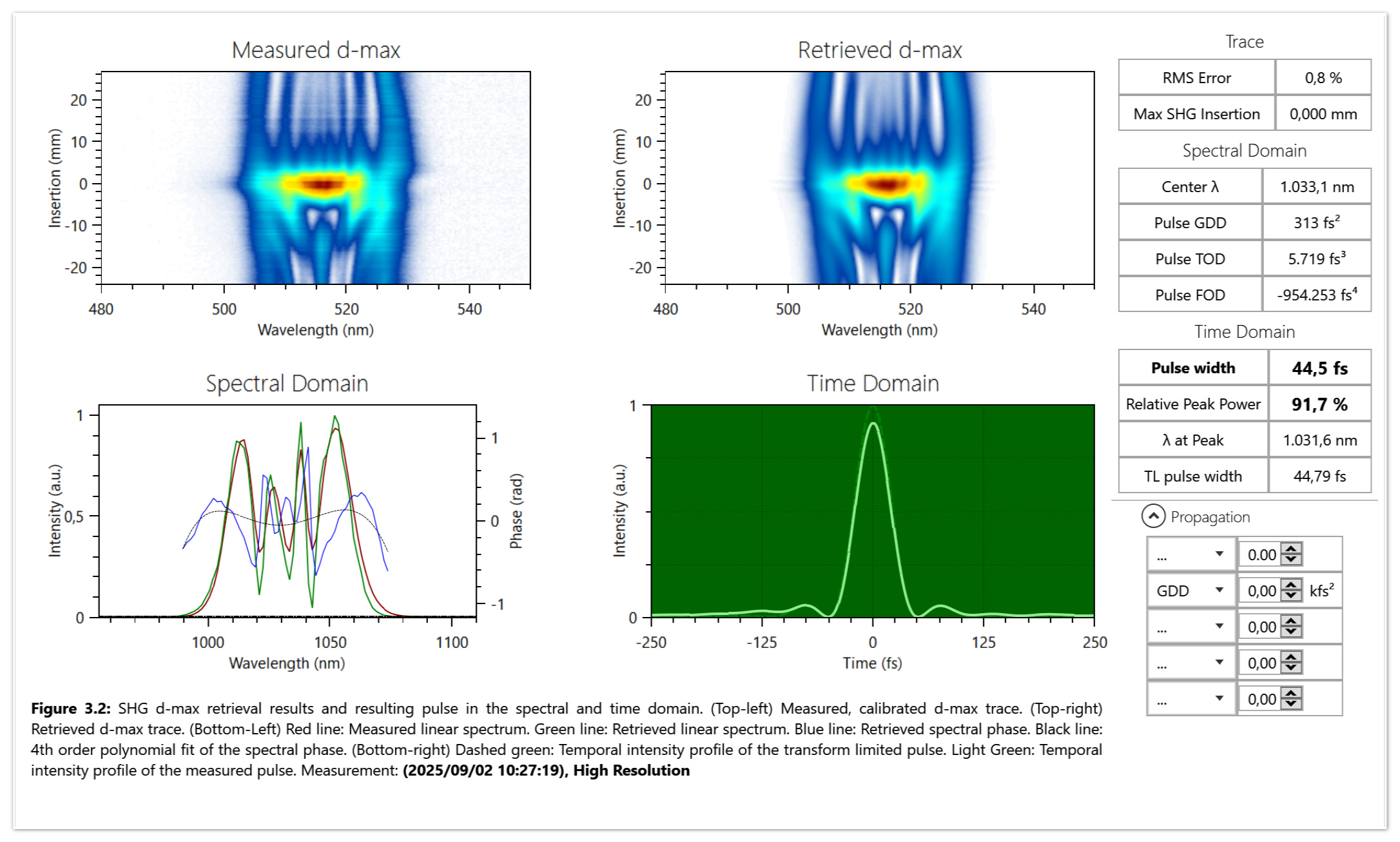
In this section, we present the performance of our MIKS1_L module with a PHAROS high-energy driver laser from Light Conversion. The compressed output pulses reach 40 fs in duration with over 90 % power transmission.
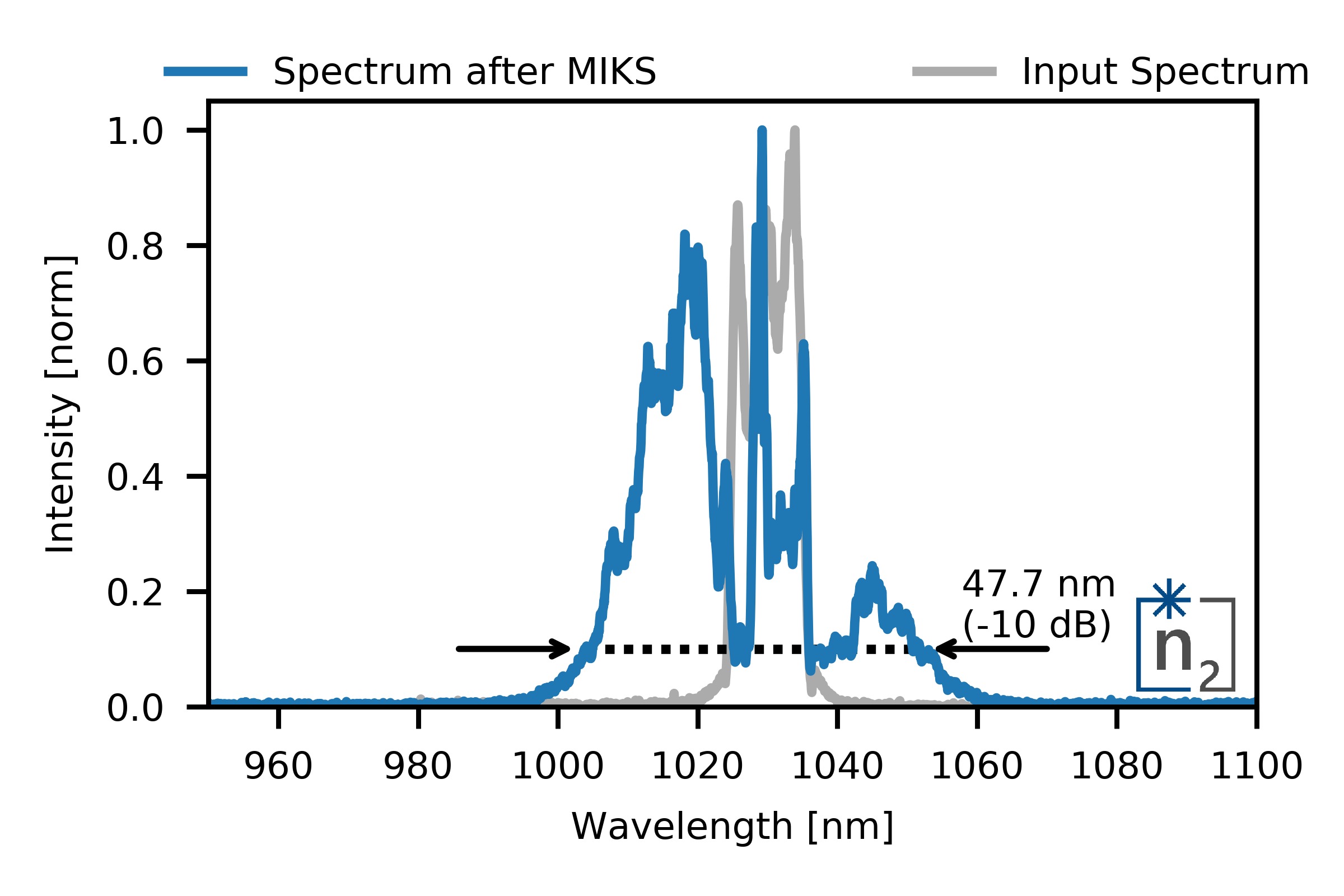
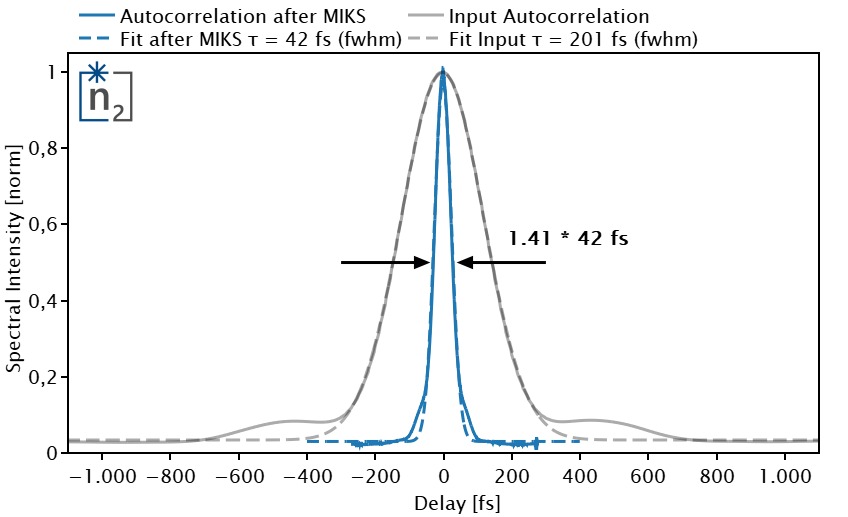
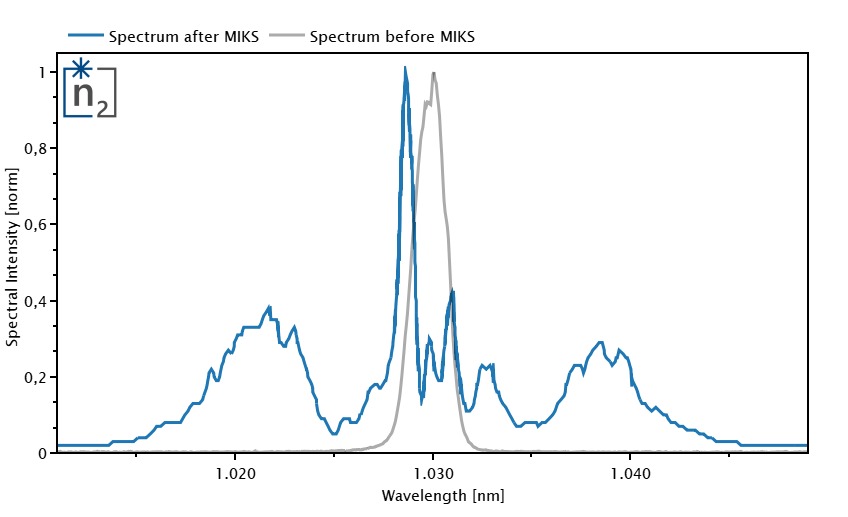
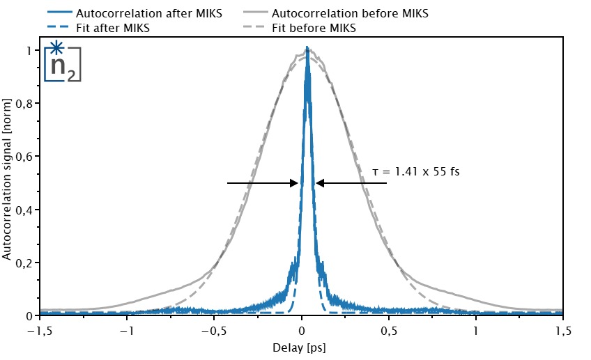
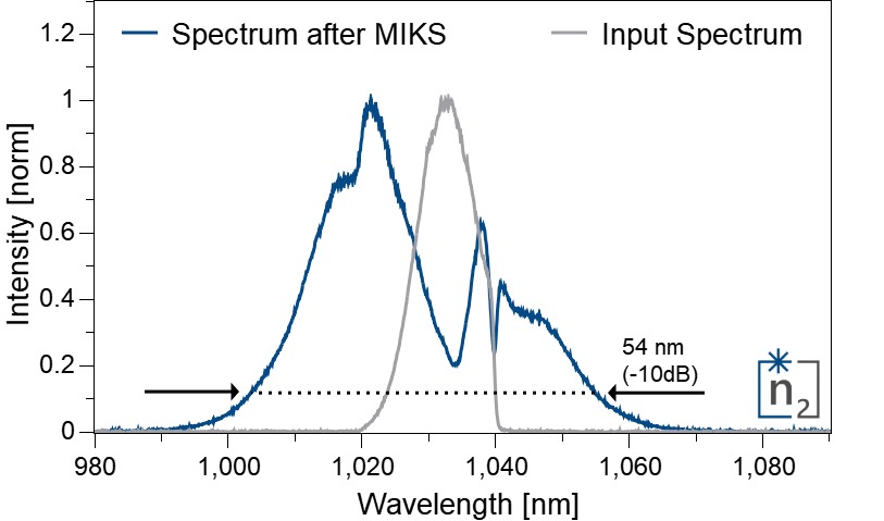
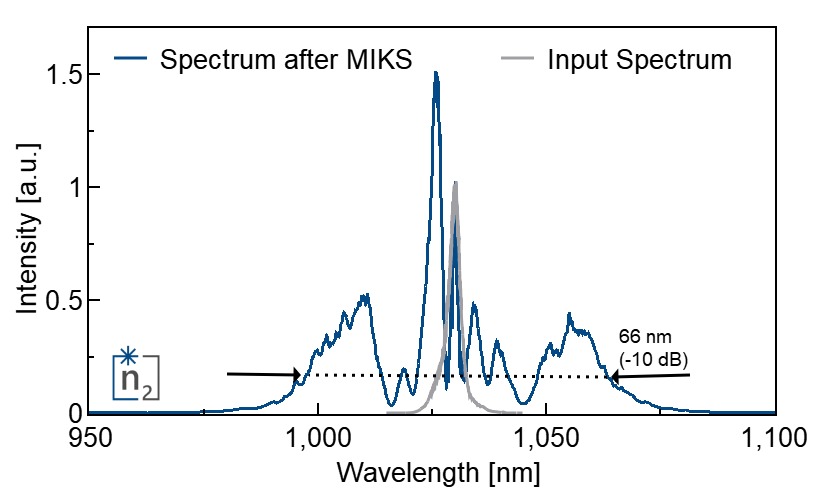
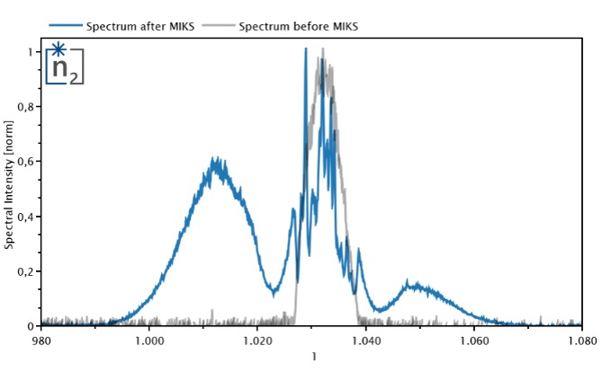
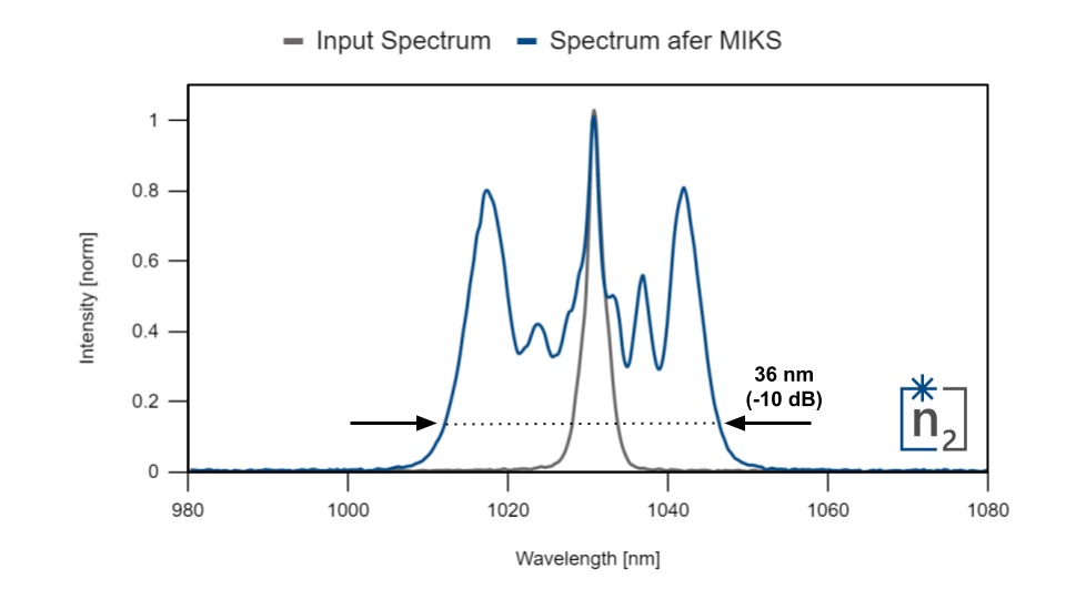
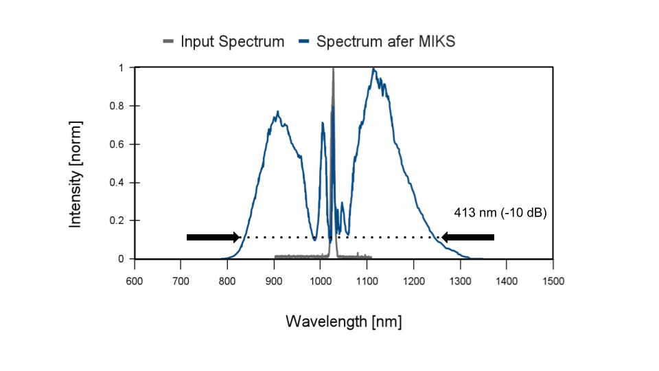
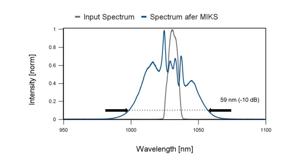
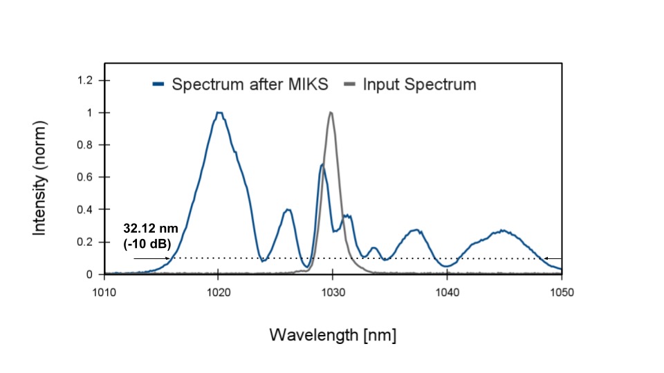
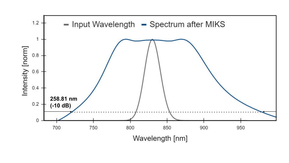
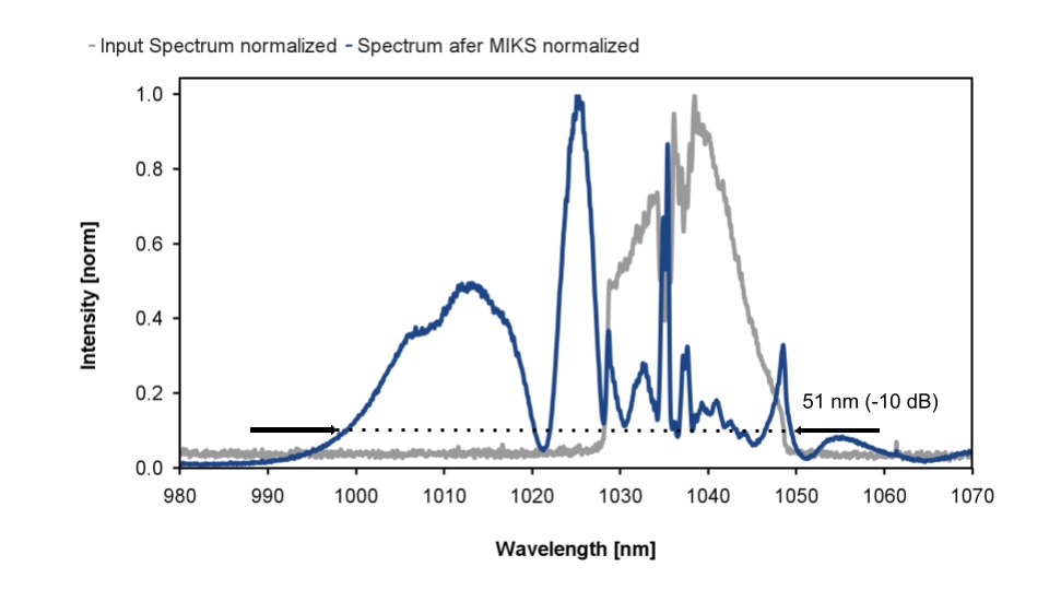
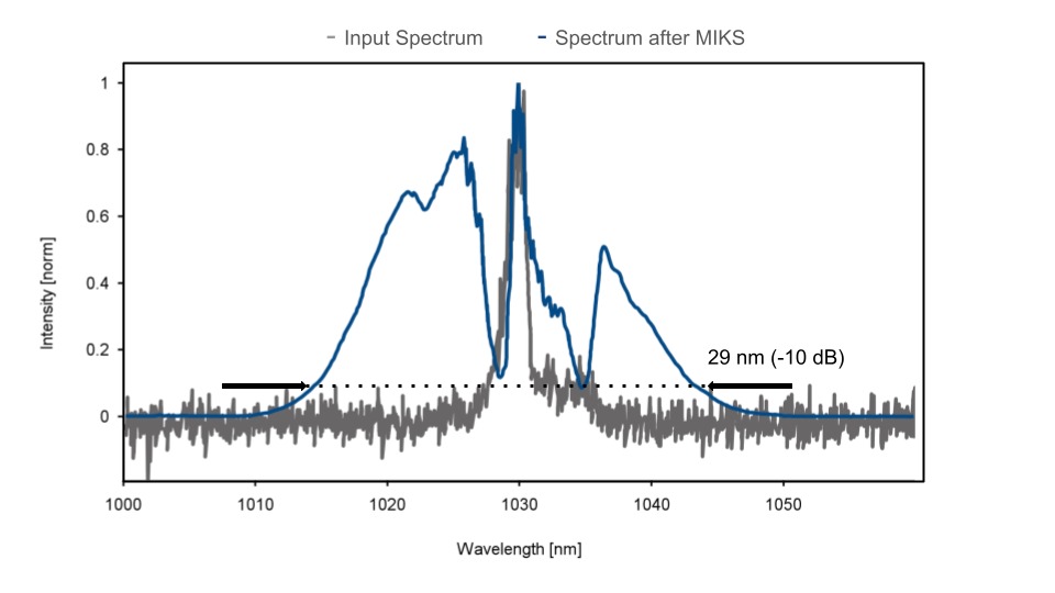
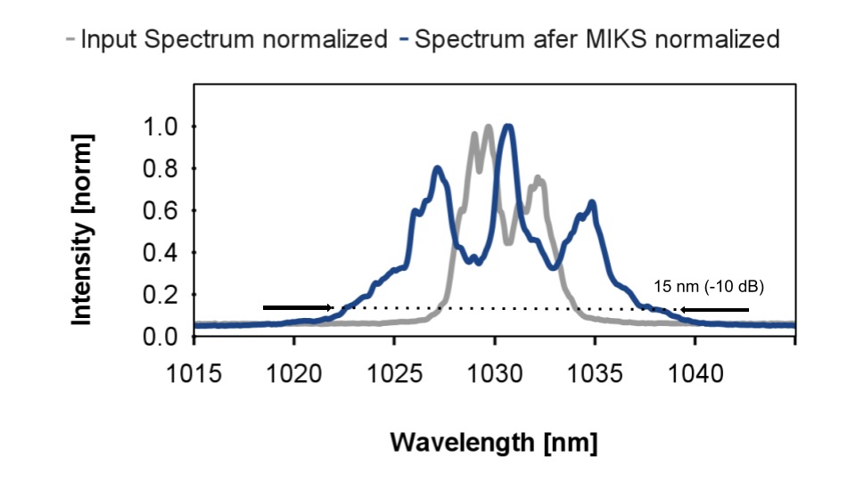
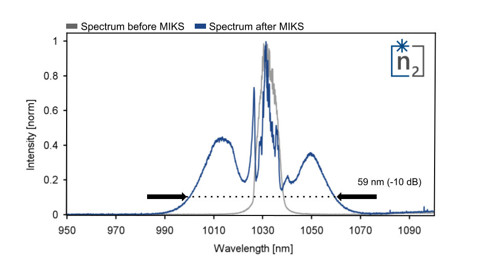
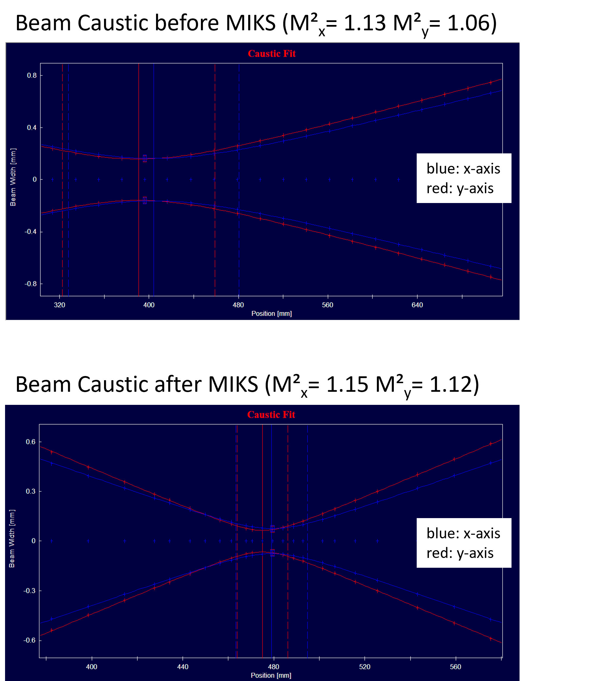
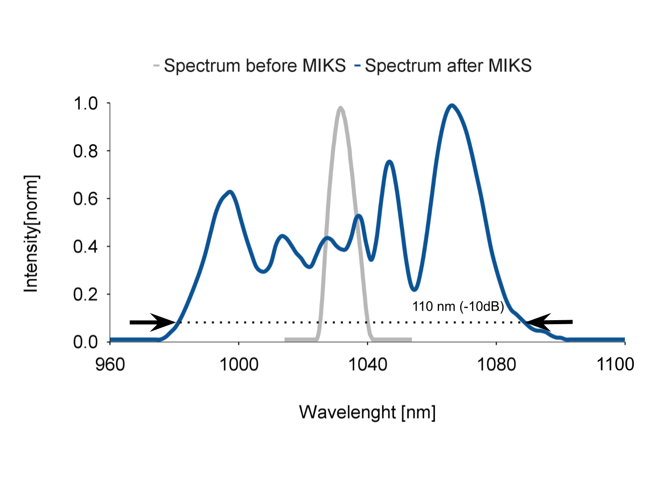
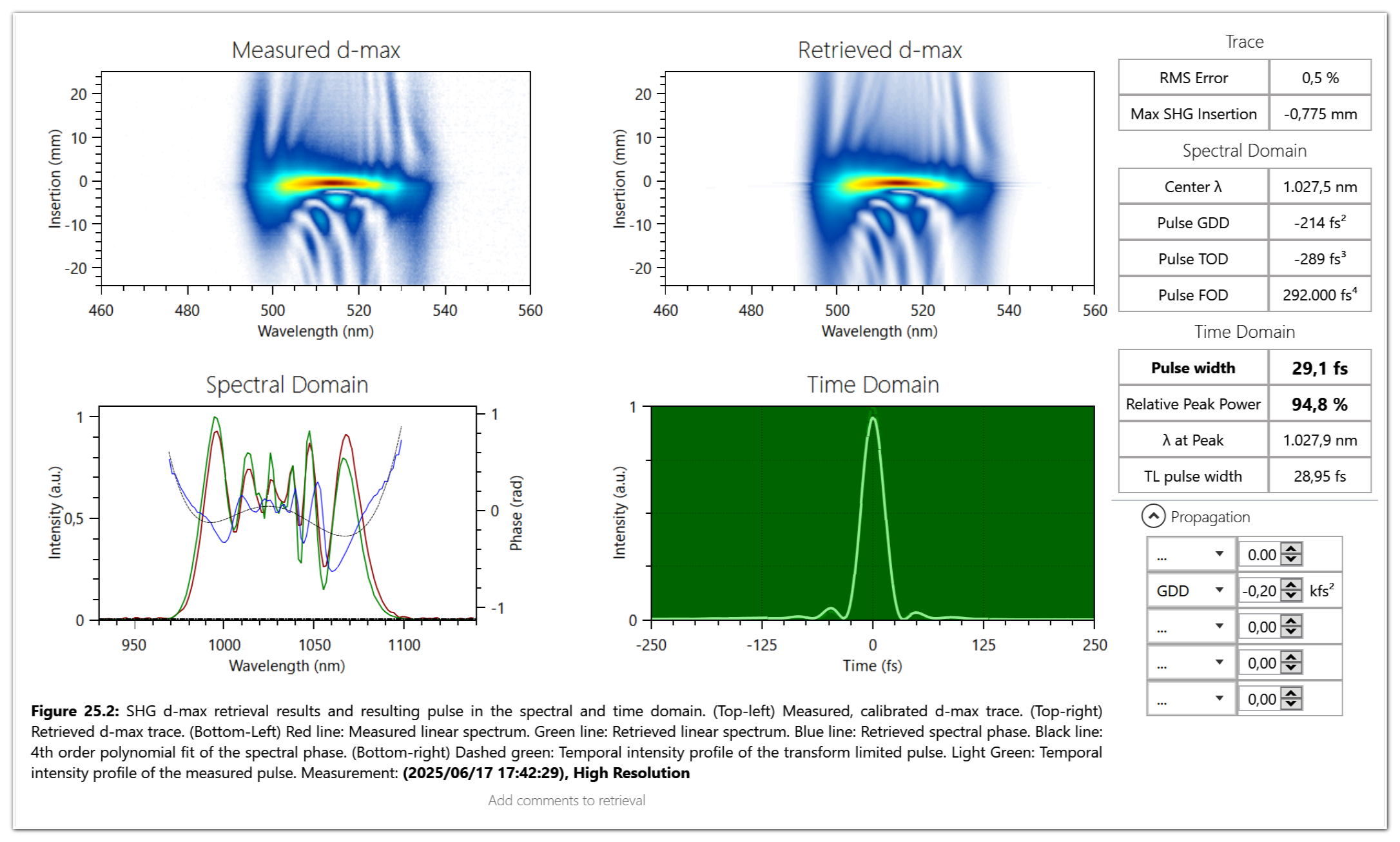
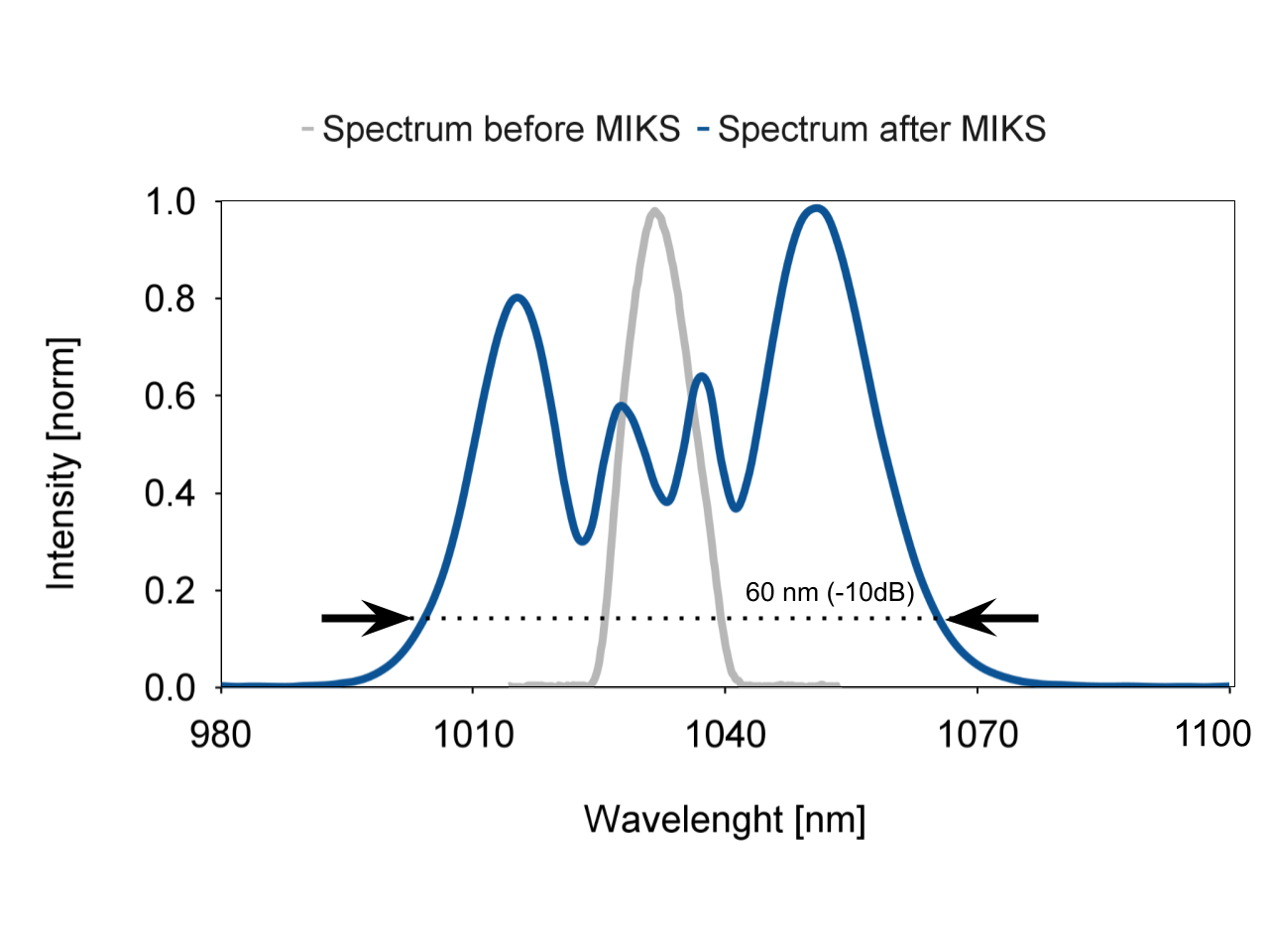
In the gas-filled multipass cell (MPC) the input spectrum is broadened via self-phase modulation to reach a Fourier-transform limit of 40 fs. Before entering the chirped mirror compressor, the pulse energy is reduced to about 10 μJ via Fresnel reflections on the front side of wedged plates.
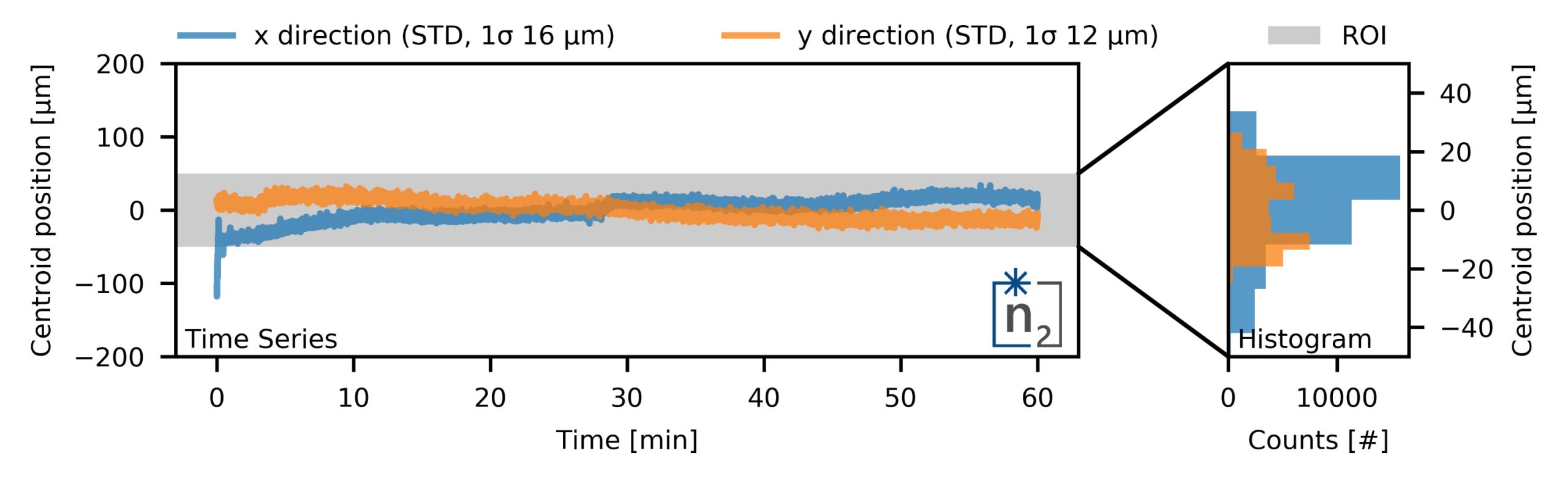
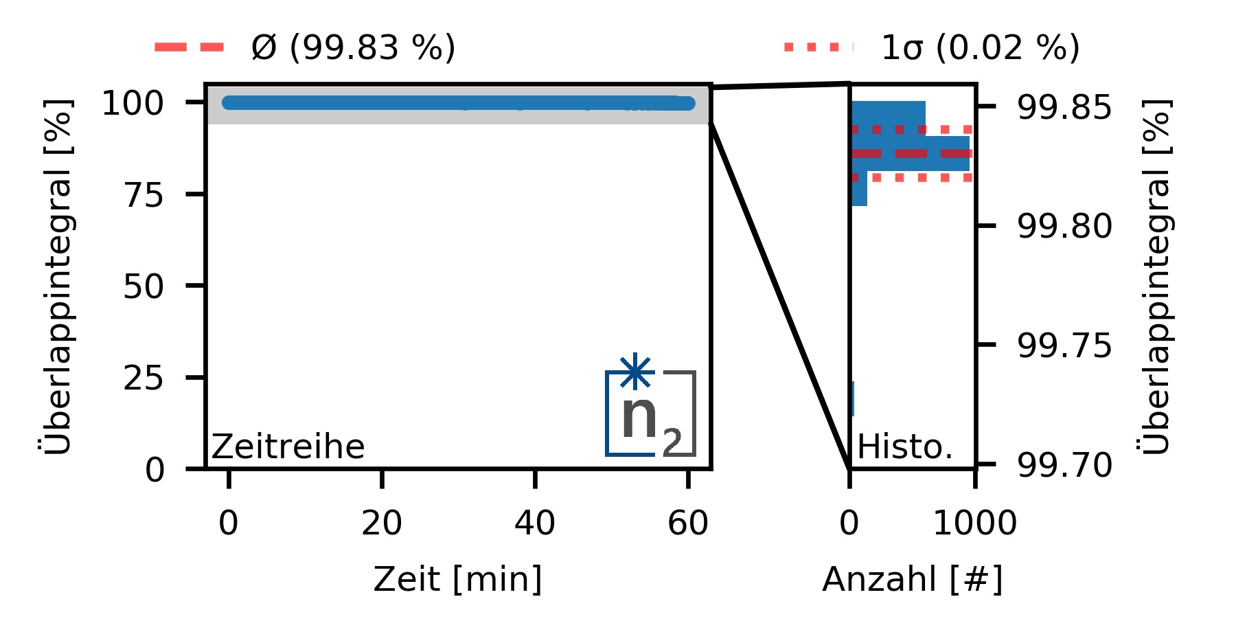
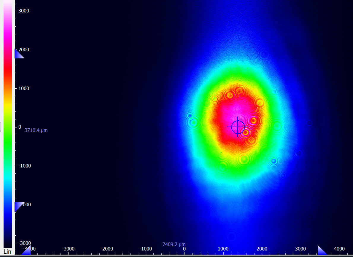
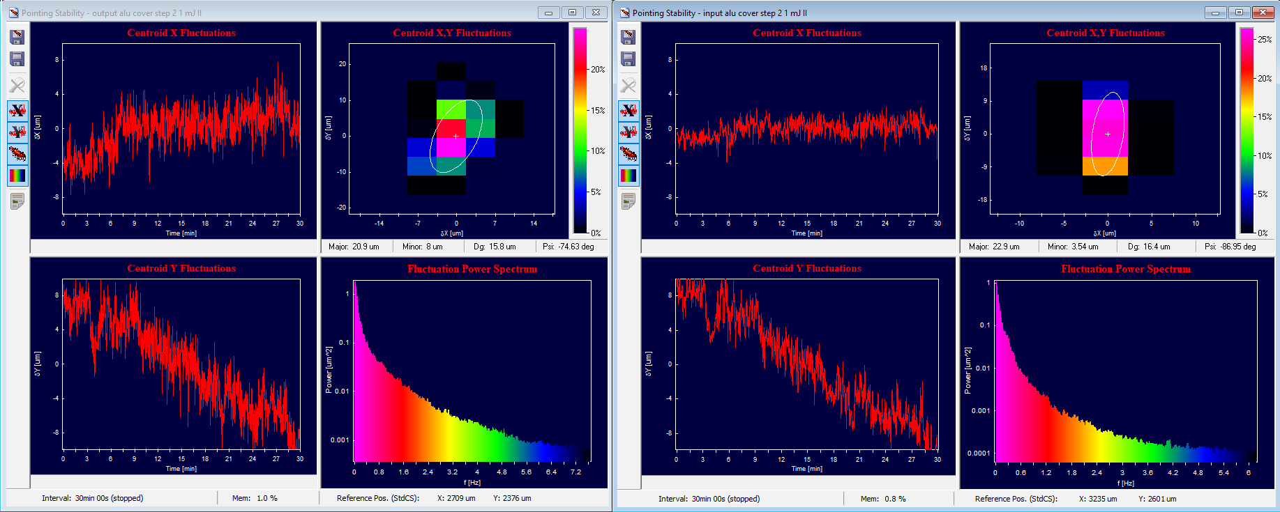
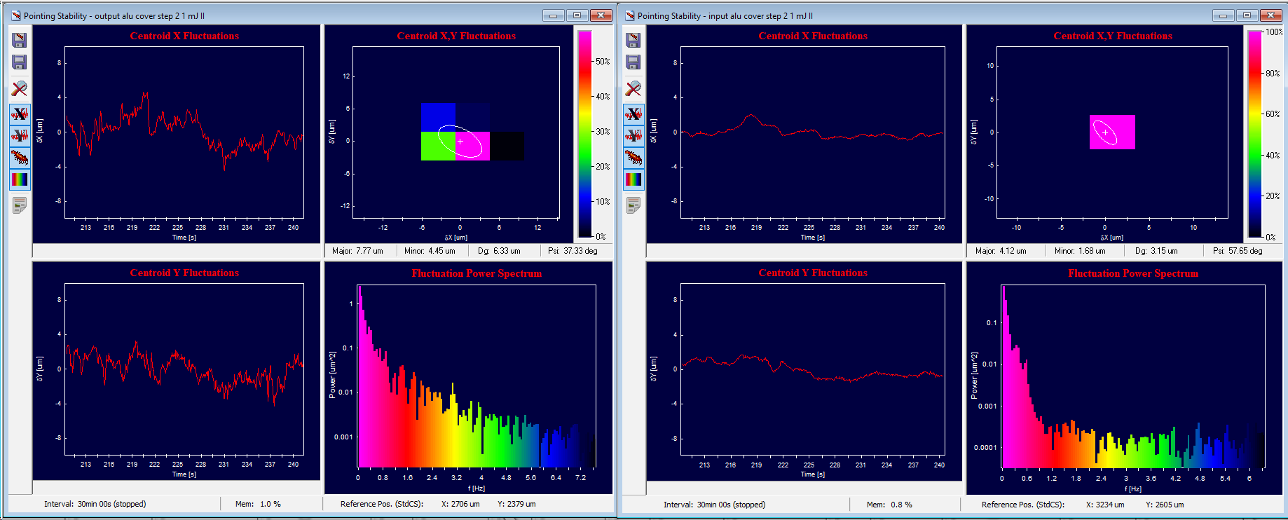
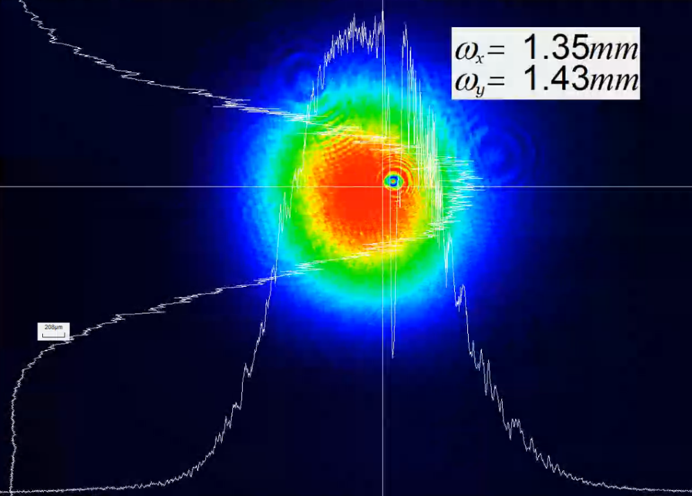
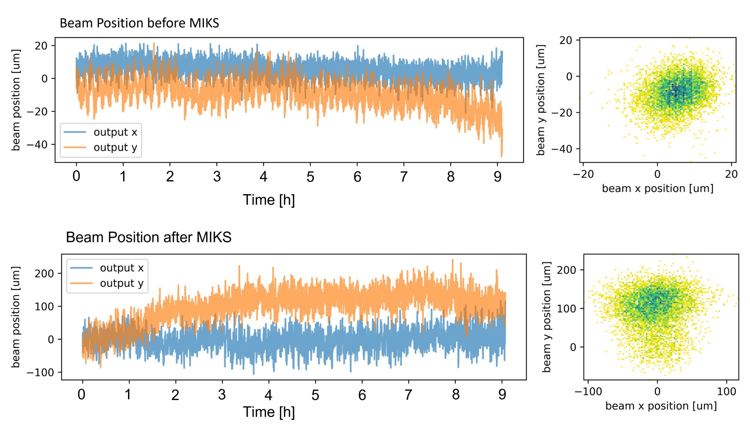
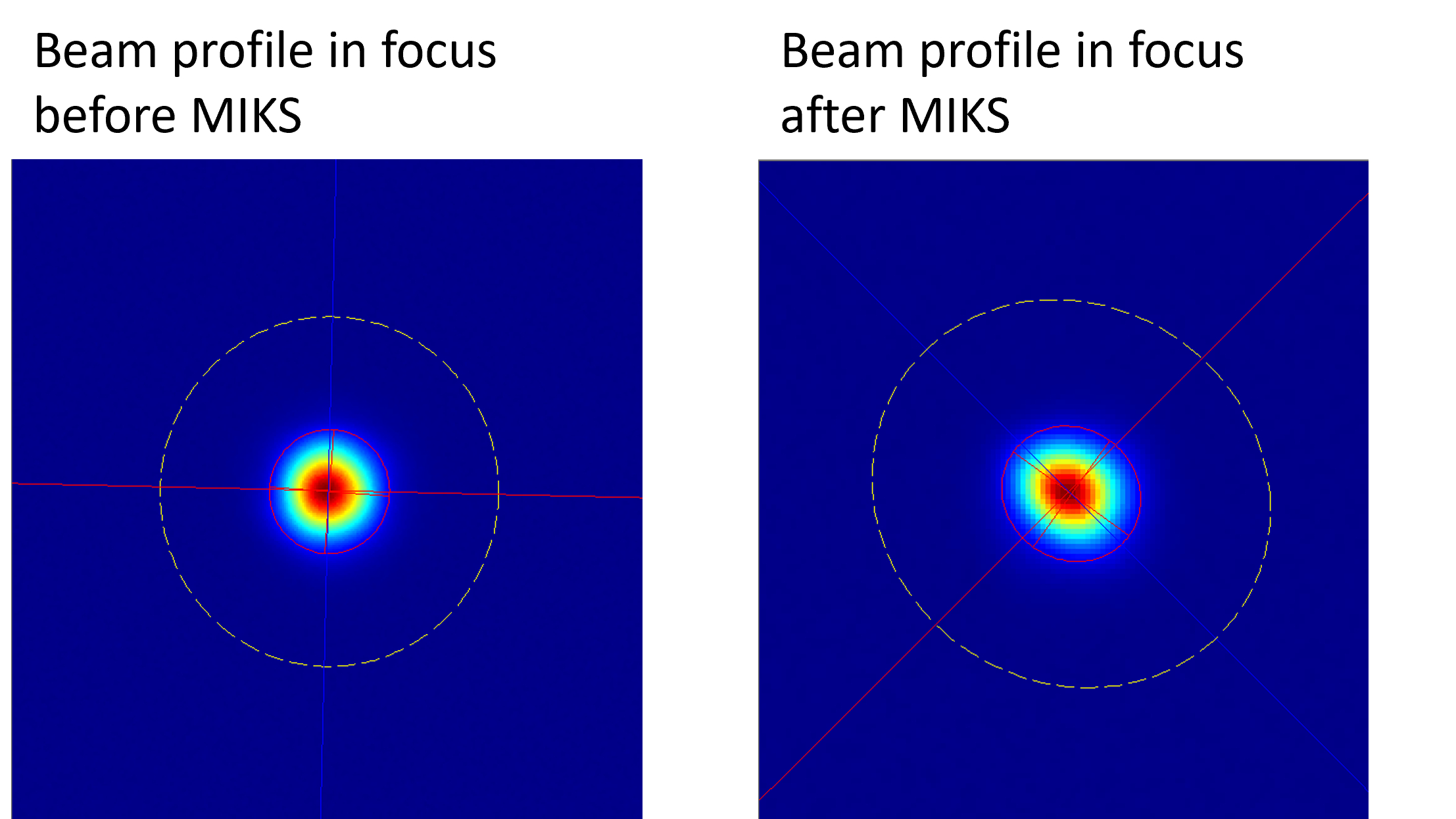
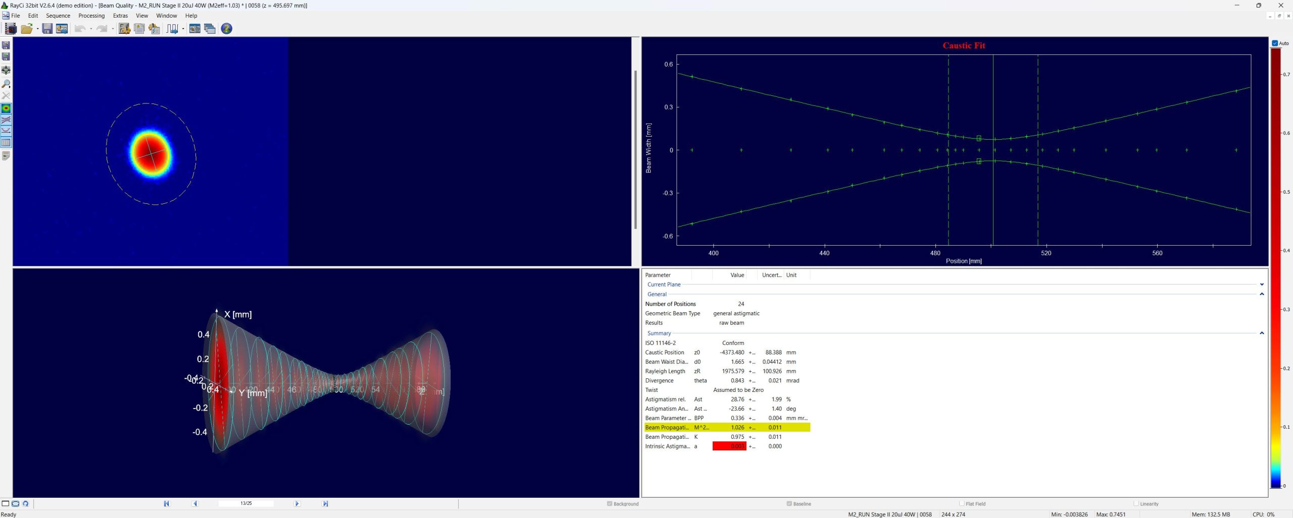
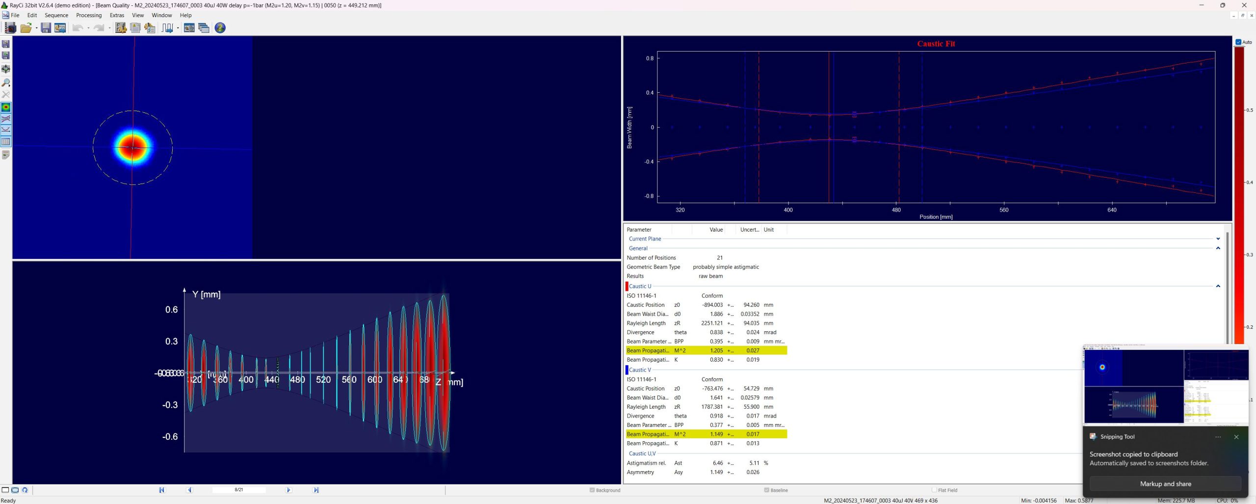
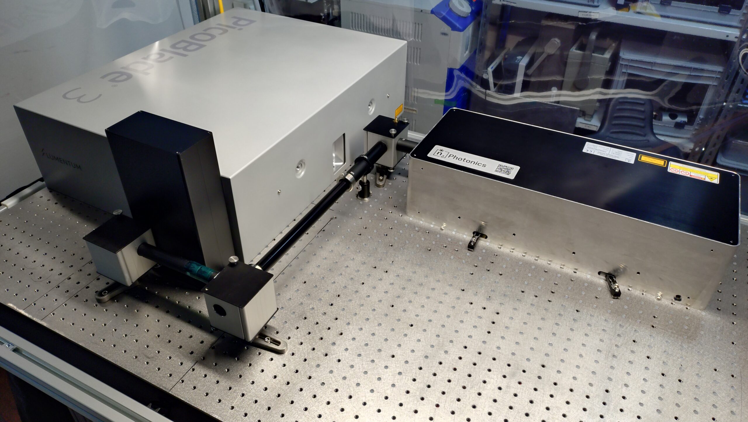
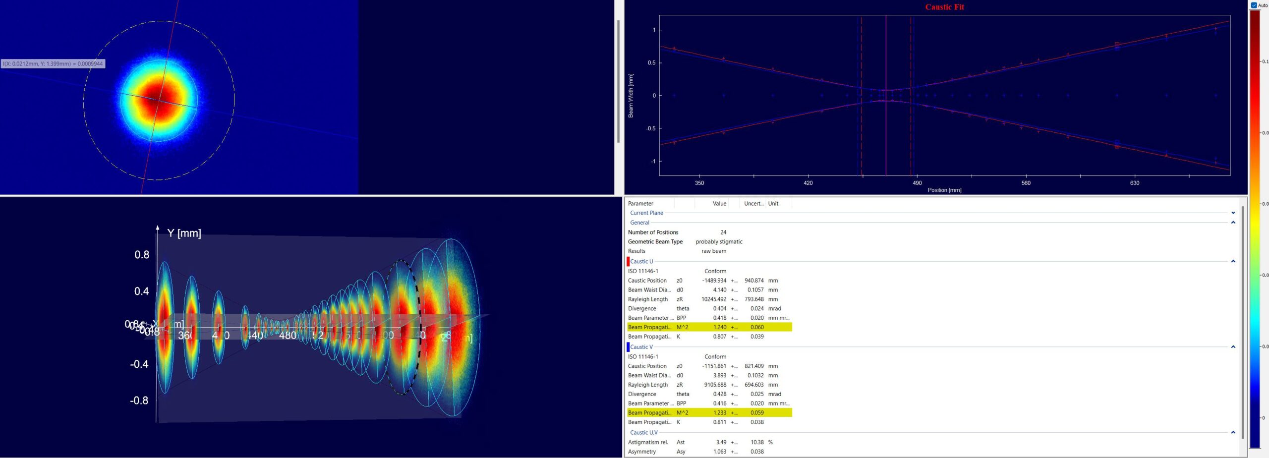
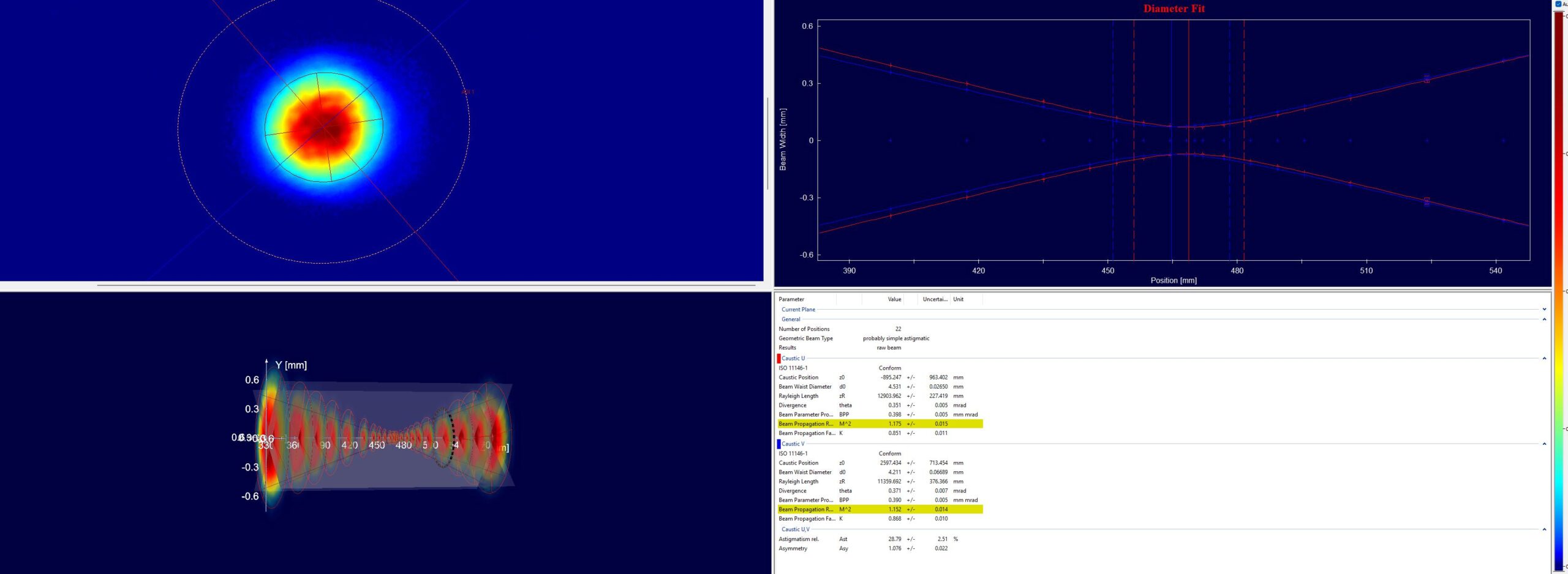
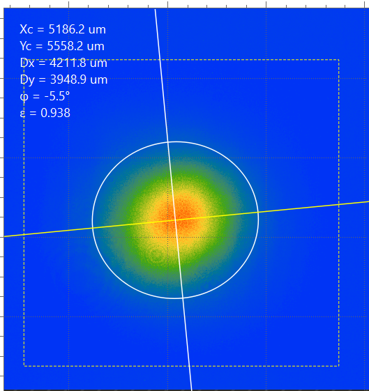
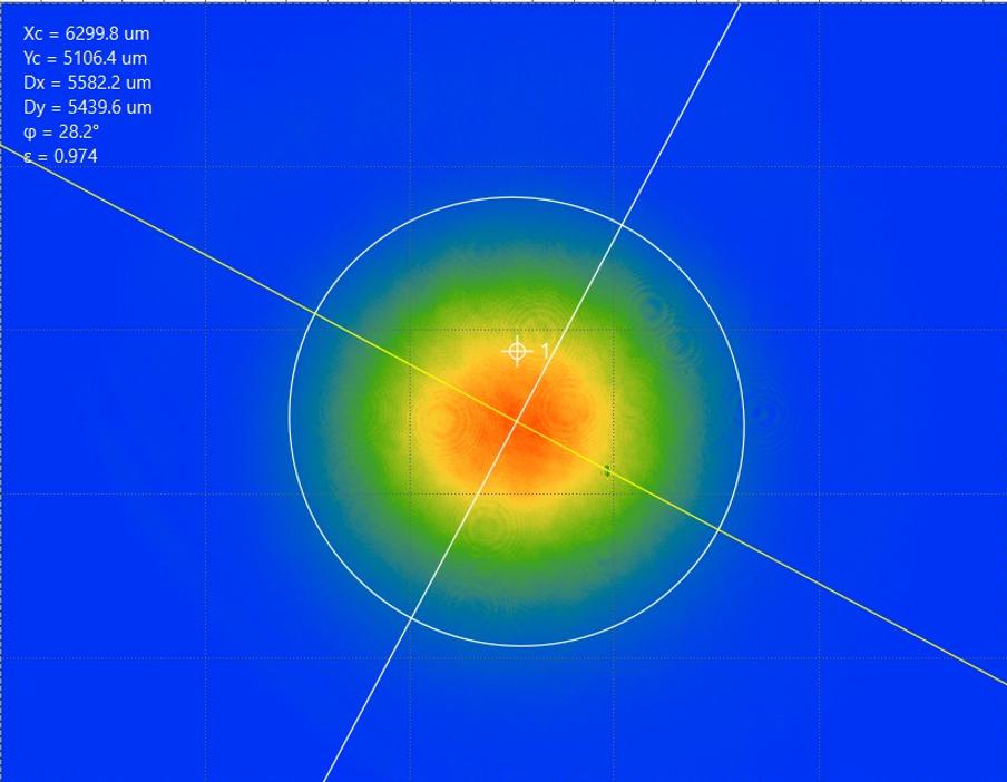
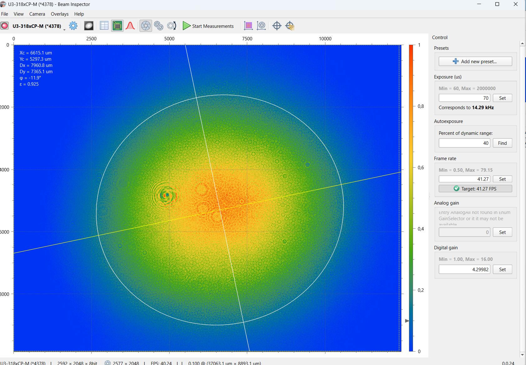
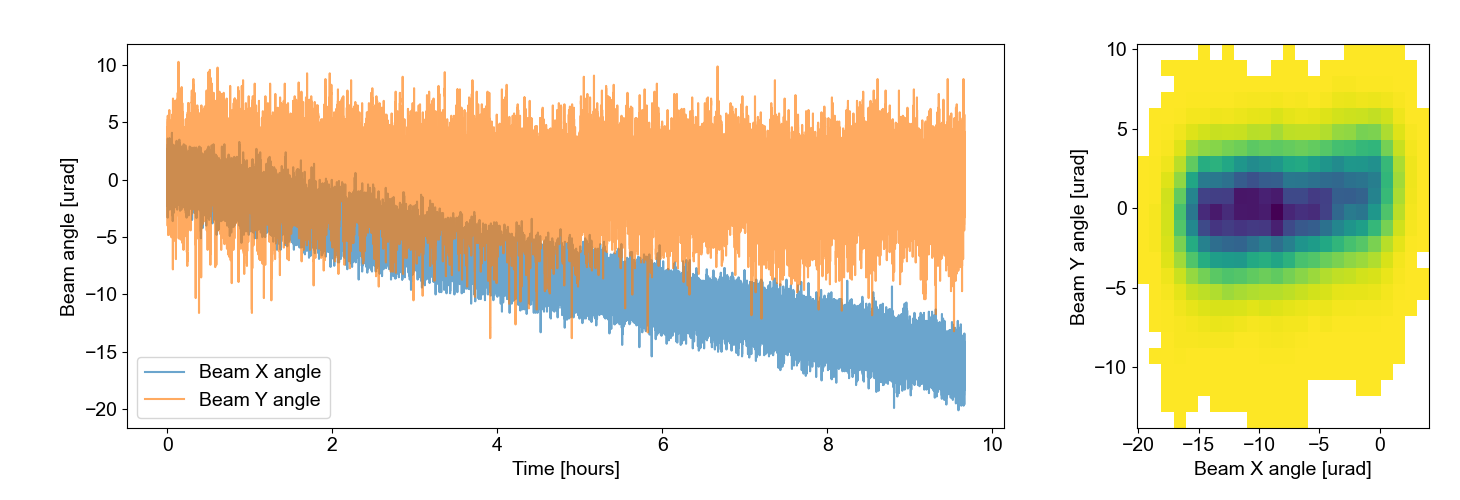
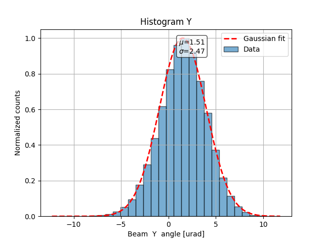
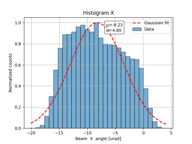
The beam pointing was measured before and after the MIKS1_L unit by two cameras in the Fourier plane of a 400 mm lens over 30 min simultaneously. It can be clearly seen that the pointing after the pulse shortening module is comparable to the pointing of the laser on that time scale with about <20 μrad. These excellent values could only be achieved by shielding the entire beam path in front of and behind the MPC from air flow as well as possible. In this particular campaign, the beam-path shielding was improvised with aluminum foil.
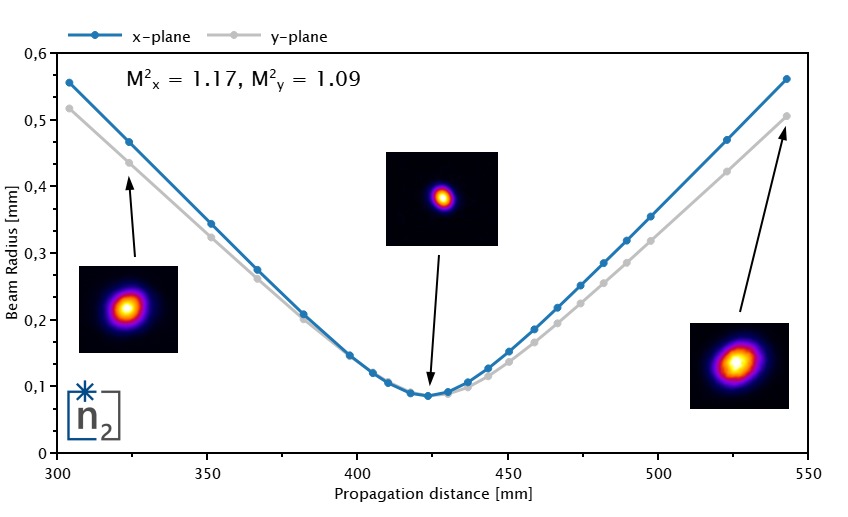
Importantly, due to limited beam time, only a small portion of the output beam was compressed to have the peak power in the compressor low and the beam size small on the chirped mirrors. For a real-world scenario, it is thus necessary to place the chirped mirror compressor as close as possible to the application to reduce the beam propagation in the air or place it directly in the experimental (vacuum) chamber.
More measurements, long long-term tests with 2 mJ/250 fs input pulses are planned. We keep improving and iterating, a lot of the presented results are work in progress.
​
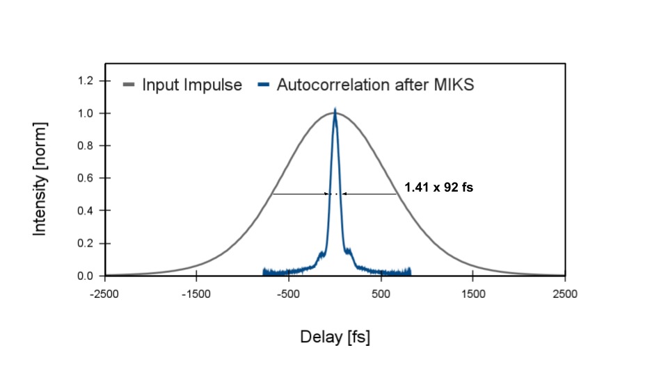
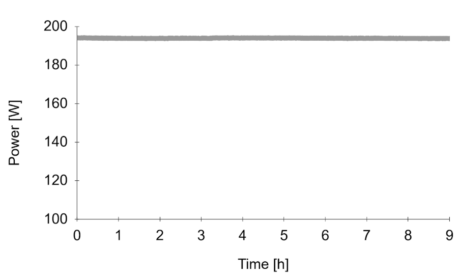
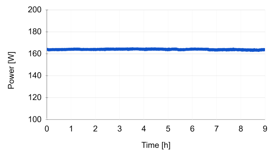
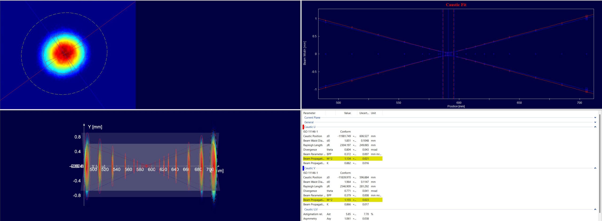
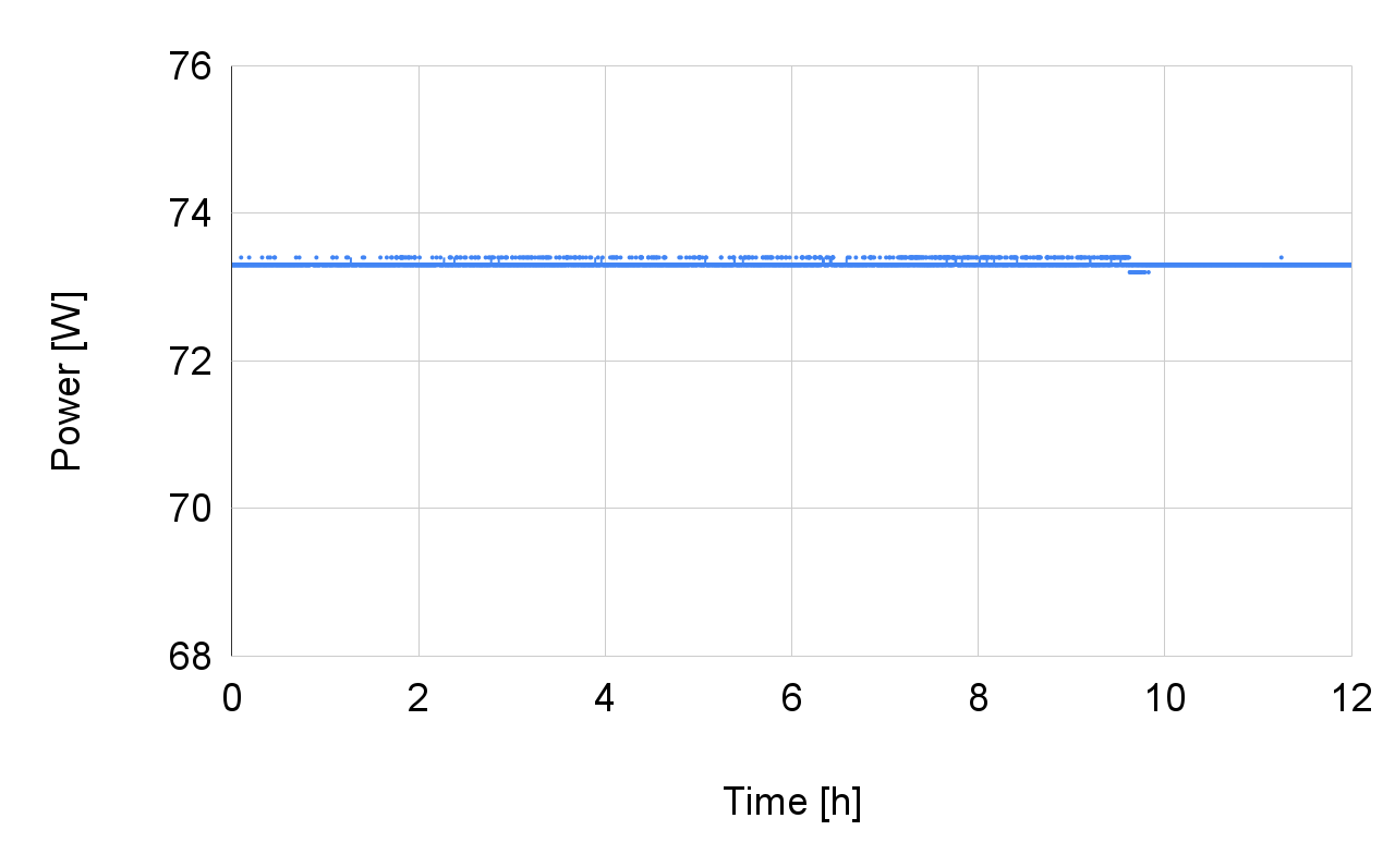
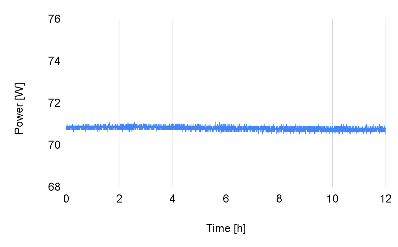
Input Pharos: 620 fs (stretched from 170 fs), 1 mJ, 10 W, 10 kHz
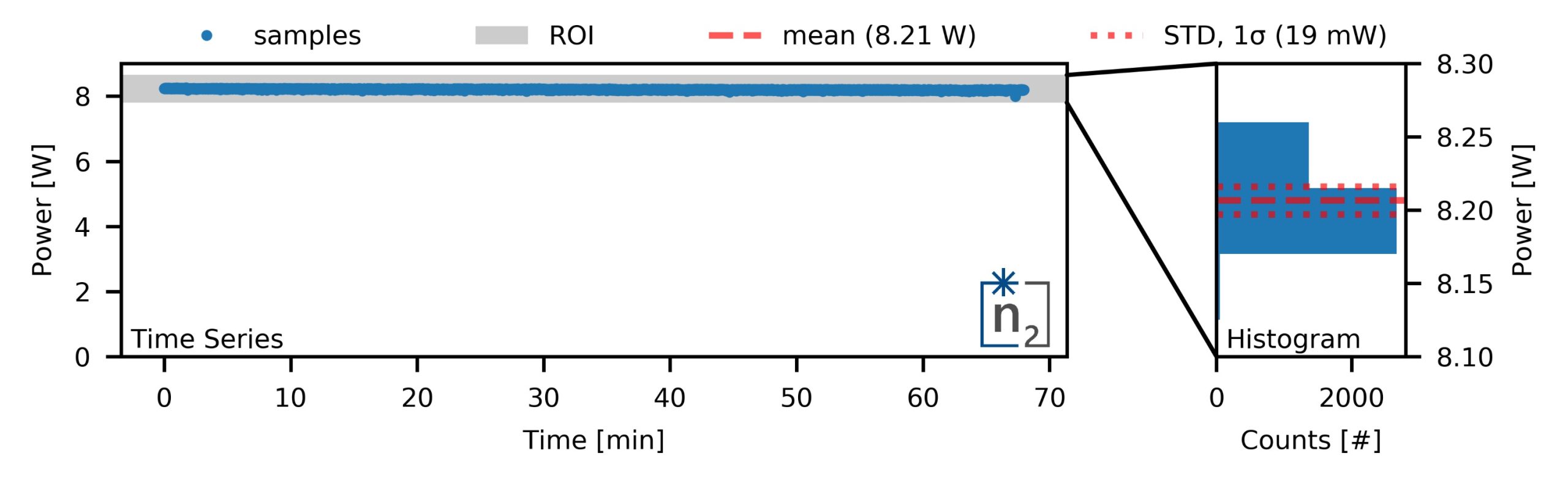
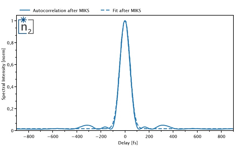
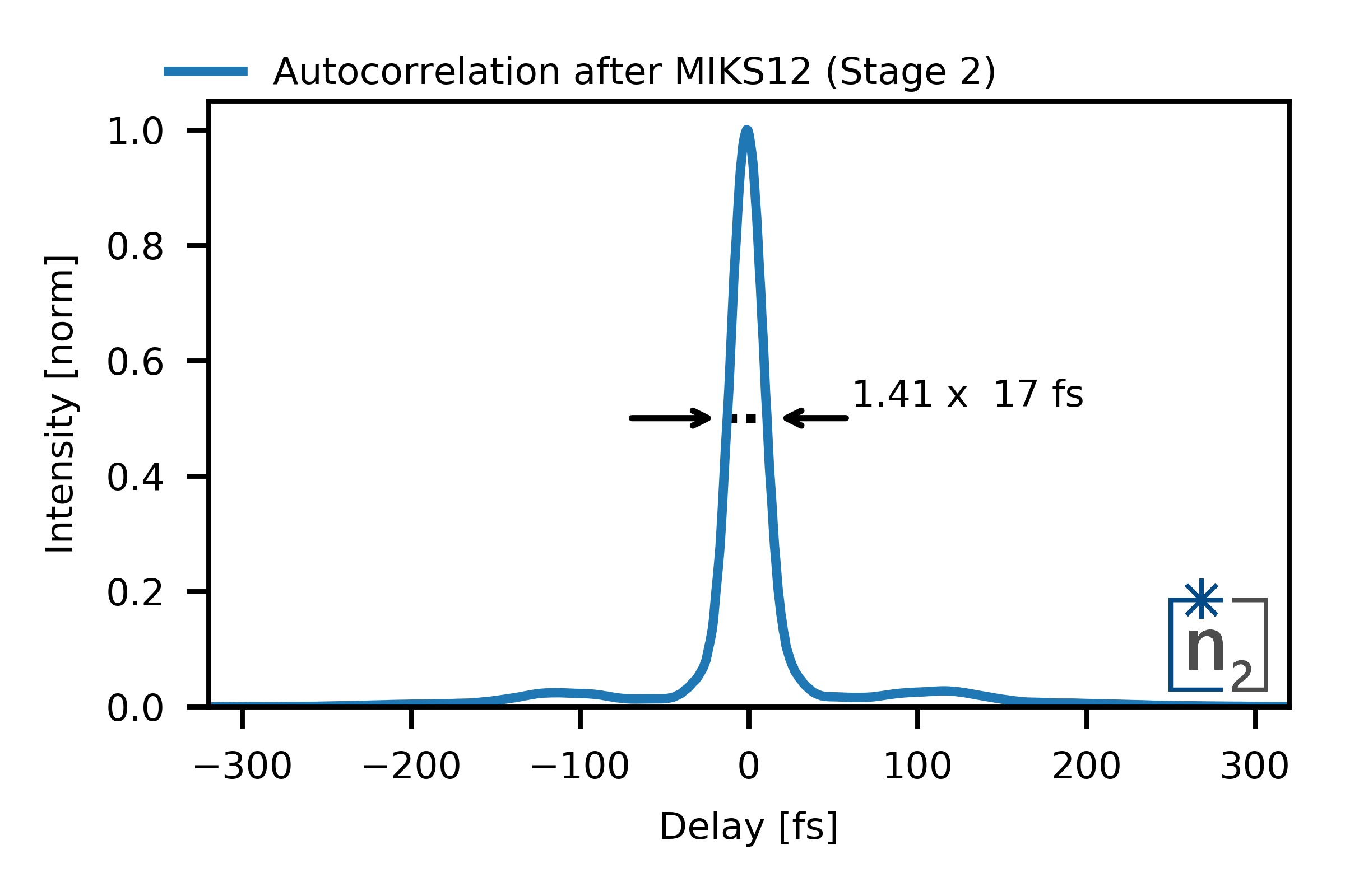
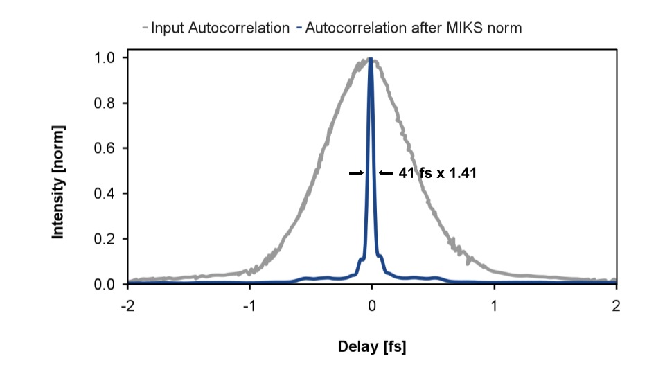
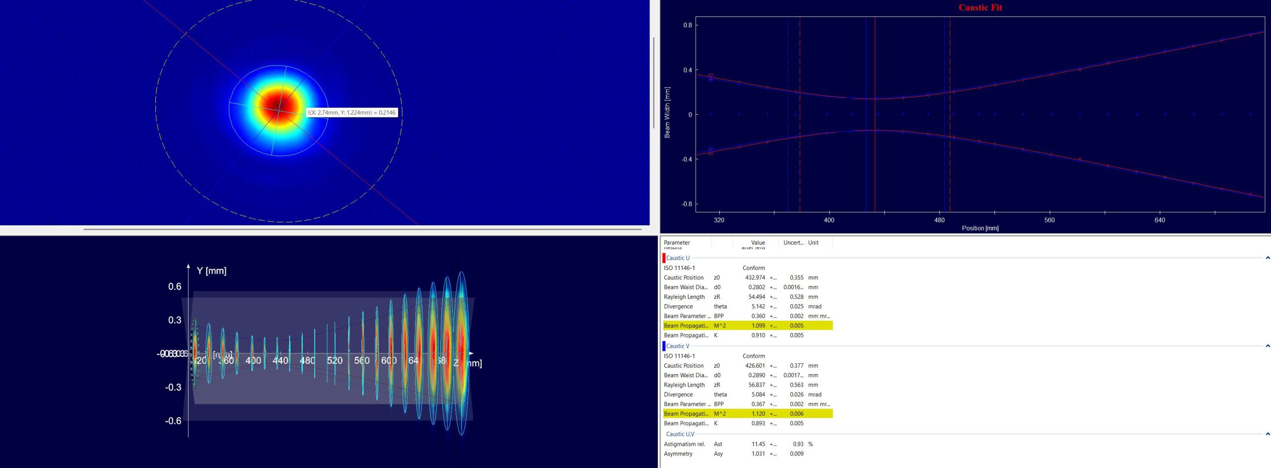
Output MIKS1_L: 41 fs, 0.98 mJ, 9.82 W
​
Input spectrum vs. output spectrum
​
Output beam profile
​
Input autocorrelation vs. output autocorrelation
​
M2 measurement
​
Beam pointing (long term, 30 min)
Left picture is output. Right picture is input.
left: Centroid fluctuation in x-direction (top), centroid fluctuation in y-direction (bottom)
right: 2D-Histogram of centroid location (top), power spectrum of centroid fluctuation (bottom)
Beam pointing (short term, 30 sec)
Left picture is output. Right picture is input.
left: Centroid fluctuation in x-direction (top), centroid fluctuation in y-direction (bottom)
right: 2D-Histogram of centroid location (top), power spectrum of centroid fluctuation (bottom)
Beam pointing stability.
The input and output beam pointing are nearly identical
​
Measurement after the pulse compressor (Left half of the screen)
-
top: Beam profile in the Fourier plane of a 400 mm lens. 1 pixel corresponds to 13 urad angle deviation
-
bottom: Beam stability analysis
-
left: Centroid fluctuation in x-direction (top), centroid fluctuation in y-direction (bottom)
-
right: 2D-Histogram of centroid location (top), power spectrum of centroid fluctuation (bottom)
-
Measurement before the pulse compressor (Right half of the screen)
-
top: Beam profile in the Fourier plane of a 400 mm lens. 1 pixel corresponds to 13 urad angle deviation
-
bottom: Beam stability analysis
-
left: Centroid fluctuation in x-direction (top), centroid fluctuation in y-direction (bottom)
-
right: 2D-Histogram of centroid location (top), power spectrum of centroid fluctuation (bottom)​
-
MIKS1_S @ Tangor (Amplitude)
​
Here we show the performance of our MIKS1_S module driven by Amplitude laser. The compressed output pulses reach 138 fs in duration with 96 % power transmission. Starting from 485 fs input pulses this corresponds to an increase in peak power of factor 3.4. The self-phase modulated spectrum and the pulse compression are shown in the graphs below.
​
Input Tangor: 485 fs, 150 uJ, 10 W
Output MIKS1_S: 138 fs, 144 µJ, 9.6 W
​
Input spectrum vs. output spectrum
​
Input autocorrelation vs. output autocorrelation
​
Output beam profile
​
MIKS1_S @ FX-Series (Edge Wave)
​
Here we show the performance of our MIKS1_S module driven by an Edge Wave femtosecond laser. A pulse duration of 220 fs could be achieved with a transmission of over 95%. The self-phase modulated spectrum and the pulse compression are shown in the graphs below.
​
Input FX-Series: 500 fs, 86 uJ, 0.86 W, 100kHz
Output MIKS1_S: 220 fs, 83 uJ, 0.83 W, 100kHz
​
Input spectrum vs. output spectrum
​
Input autocorrelation vs. output autocorrelation
​
Output beam profile
​
MIKS1_S @ Satsuma (Amplitude)
​
In this section we present the performance of our multipass cell spectral broadening and compression module with Satsuma Amplitude driving laser. The 290 fs pulses from Satsuma laser are compressed down to 50 fs in duration with over 95 % power transmission. Starting from 290 fs input pulses this leads to nearly 5-6 times increased output peak power.
​
Input Satsuma: 19.8 W , 40 µJ , 287 fs
Output MIKS1_S: 19.6 W, 39 µJ, 49 fs
​
Input spectrum vs. output spectrum
​
Input autocorrelation vs output autocorrelation
​
Beam pointing/positional stability
​
Output power stability
​
Beam profile
​
Beam Caustic and M²
​